The last installment talked about the GJK algorithm as it pertains to collision detection. The original algorithm actually is used to obtain the distance and closest points between two convex shapes.
Introduction
The algorithm uses much of the same concepts to determine the distance between the shapes. The algorithm is iterative, uses the Minkowski Sum/Difference, looks for the origin, and uses the same support function.
Overview
We know that if the shapes are not colliding that the Minkowski Difference will not contain the origin. Therefore instead of iteratively trying to enclose the origin with the simplex, we will want to generate a simplex that is closest to the origin. The closest simplex will always be on the edge of the Minkowski Difference. The closest simplex for 2D could be either a single point or a line.
Minkowski Sum
Just as we did for the collision detection portion of GJK in the previous post, the algorithm also needs to know the Minkowski Sum (Difference is what I will call it, see the GJK post).
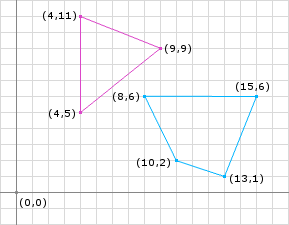
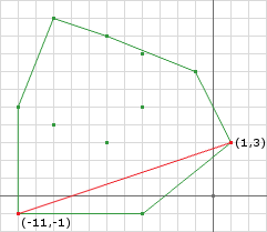
Taking the same shapes from the GJK post and separating them (Figure 1) yeilds the same Minkowski Difference only translated slightly (Figure 2). We notice that the origin is not contained within the Minkowski Difference, therefore there is not a collision.
The Distance
The distance can be calculated by finding the closest point on the Minkowski Difference to the origin. The distance is then the magnitude of the closest point. By inspection, we see that the edge created by the points (-4, -1) and (1, 3) is the closest feature to the origin. Naturally the closest point to the origin is the point on this edge that forms a right angle to the origin. We can calculate the point by:
A = (-4, -1)
B = (1, 3)
// create the line
AB = (1, 3) - (-4, -1) = (5, 4)
AO = (0, 0) - (-4, -1) = (4, 1)
// project AO onto AB
AO.dot(AB) = 4 * 5 + 1 * 4 = 24
// get the length squared
AB.dot(AB) = 5 * 5 + 4 * 4 = 41
// calculate the distance along AB
t = 24 / 41
// calculate the point
AB.mult(t).add(A) = (120 / 41, 96 / 41) + (-4, -1)
                  = (-44 / 41, 55 / 41)
                  ≈ (-1, 1.3)
d = (-1, 1.3).magnitude() ≈ 1.64
This is a simple calculation since we know what points of the Minkowski Difference to use.
Iteration
Like the collision detection routine of GJK the distance routine is iterative (and almost identical for that matter). We need to iteratively build a simplex which contains the closest points on the Minkowski Difference to the origin. The points will be obtained using a similar method of choosing a direction, using the support function, and checking for the termination case.
Lets examine some psuedo code:
// exactly like the previous post, use whatever
// initial direction you want, some are more optimal
d = // choose a direction
// obtain the first Minkowski Difference point using
// the direction and the support function
Simplex.add(support(A, B, d));
// like the previous post just negate the
// the prevous direction to get the next point
Simplex.add(support(A, B, -d));
// start the loop
while (true) {
  // obtain the point on the current simplex closest
  // to the origin (see above example)
  p = ClosestPointToOrigin(Simplex.a, Simplex.b);
  // check if p is the zero vector
  if (p.isZero()) {
    // then the origin is on the Minkowski Difference
    // I consider this touching/collision
    return false;
  }
  // p.to(origin) is the new direction
  // we normalize here because we need to check the
  // projections along this vector later
  d = p.negate().normalize();
  // obtain a new Minkowski Difference point along
  // the new direction
  c = support(A, B, d);
  // is the point we obtained far enough along d?
  double dc = c.dot(d);
  // you can use a or b here it doesn't matter
  double da = Simplex.a.dot(d);
  // tolerance is how acurate you want to be
  if (dc - da < tolerance) {
    // if we got closer, given some tolerance,
    // to the origin, then we can assume that we
    // are done
    distance = dc;
    return true;
  }
  // if we are still getting closer then only keep
  // the points in the simplex that are closest to
  // the origin (we already know that c is closer
  // than both a and b)
  // the magnitude is the same as distance(origin, a)
  if (a.magnitude() < b.magnitude()) {
    b = c;
  } else {
    a = c;
  }
}
The first few lines look a lot like the previous GJK post. The difference is the building of our simplex. We are using the same idea of a simplex, we use the same support function and roughly the same logic, however, we only keep 2 points at all times (3D would be 3 points) and we find a point on the simplex closest to the origin instead of finding the Voronoi region that the origin lies in.
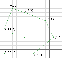
As we did in the previous post this is best explained by running through an example. Let’s take the example above from Figure 1 and run through the iterations.
Pre Iteration:
// im going to choose the vector joining the
// centers of the objects as the initial d
d = (11.5, 4.0) - (5.5, 8.5) = (6, -4.5)
Simplex.add(support(A, B, d)) = (9, 9) - (8, 6) = (1, 3)
Simplex.add(support(A, B, -d)) = (4, 11) - (13, 1) = (-9, 10)
// start the iterations
Iteration 1:
// find the new d
// by inspection we can tell that (1, 3) is the closest
// the computation will yield the same result
p = (1, 3)
d = (-1, -3) ≈ (-0.32, -0.95)
// get a new point in this direction
c = support(A, B, d) = (4, 5) - (15, 6) = (-11, -1)
// is c far enough along d
dc = 3.52 + 0.95 = 4.47
da = -0.32 - 2.85 = -3.17
// 4.47 - -3.17 = 7.64 not small enough
maga = a.magnitude() = 3.16
magb = b.magnitude() = 13.45
// a is smaller so replace b with c
b = c
In this first iteration I didn’t go through the trouble of calculating p because its obviously going to be the end point a. If you performed the real calculation, like the code will do, you will obtain the same result. We notice that even though the closest point is a point already on the simplex, we can still use it as the next direction. We obtain a new point using the new direction and keep the two closest points.
Iteration 2:
// find the new d
// by inspection we can tell that we need to perform
// the closest point computation
a = (1, 3)
b = (-11, -1)
AB = (-11, -1) - (1, 3) = (-12, -4)
AO = (0, 0) - (1, 3) = (-1, -3)
AO.dot(AB) = -1 * -12 + -3 * -4 = 24
AB.dot(AB) = -12 * -12 + -4 * -4 = 160
t = 24 / 160 = 3 / 20
p = AB.mult(t).add(A) = (-36/20, -12/20) + (1, 3) = (-4/5, 12/5)
d ≈ (0.8, -2.4) ≈ (0.32, -0.95)
// get a new point in this direction
c = support(A, B, d) = (4, 5) - (8, 6) = (-4, -1)
// is c far enough along d
dc = -1.28 + 0.95 = -0.33
da = 0.32 - 2.85 = -2.53
// -0.33 - -2.53 = 2.2 not small enough
maga = a.magnitude() = 3.16
magb = b.magnitude() = 11.05
// a is smaller so replace b with c
b = c
Notice that our simplex is getting closer to the origin.
Iteration 3:
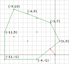
// find the new d
// by inspection we can tell that we need to perform
// the closest point computation
a = (1, 3)
b = (-4, -1)
AB = (-4, -1) - (1, 3) = (-5, -4)
AO = (0, 0) - (1, 3) = (-1, -3)
AO.dot(AB) = -1 * -5 + -3 * -4 = 17
AB.dot(AB) = -5 * -5 + -4 * -4 = 41
t = 17 / 41
p = AB.mult(t).add(A) = (-85/41, -68/20) + (1, 3) = (-44/41, 55/41)
d ≈ (-1.07, 1.34) ≈ (0.62, -0.78)
// get a new point in this direction
c = support(A, B, d) = (9, 9) - (8, 6) = (1, 3)
// is c far enough along d
dc = 0.62 - 2.34 = -1.72
da = 0.62 - 2.34 = -1.72
// -1.72 - -1.72 = 0 i think thats small enough!
// we done!
distance = 1.72
We notice that when we terminated the difference in projections was zero. This can only happen with two polygons. If either A or B was a shape with a curved edge the difference in projections would approach zero but not obtain zero. Therefore we use a tolerance to handle curved shapes since the tolerance will also work for polygons.
Another problem curved shapes introduce is that if the chosen tolerance is not large enough the algorithm will never terminate. In this case we add a maximum iterations termination case.
One more problem that this algorithm can run into is if the shapes are actually intersecting. If they are intersecting the algorithm will never terminiate. This isn’t as big of a problem since most of the time you will determine if the shapes are colliding first anyway. If not, then we must add a check in the while loop for the simplex containing the origin. This can be done by a simple point in triangle test (2D).
Closest Points
In addition to the distance between the two shapes, we can also determine the closest points on the shapes. To do this we need to store additional information as we progress through the algorithm. If we store the points on the shapes that were used to create the Minkowski Difference points we can use them later to determine the closest points.
For instance, we terminated above with the Minkowski Difference points A = (1, 3) and B = (-4, -1). These points were created by the following points on their respective shapes:
| Shape Points | |||
|---|---|---|---|
| S1 | S2 | Minkowski Point | |
| A | (9, 9) | (8, 6) | = (1, 3) |
| B | (4, 5) | (8, 6) | = (-4, -1) |
The points used to create the Minkowski Difference points are not necessarily the closest points. However, using these source points we can calculate the closest points.
Convex Hull
We see that the points from A and B are not the correct closests points. By inspection we can see that the closest point on B is (8, 6) and the closest point on A is roughly (6.75, 7.25). We must do some calculation to obtain the closest points. Here’s where the definition of a Convex Hull comes in:
CH(S) = ∑i=1…n λiPi = λ1P1 + … + λnPn
where Pi∈S, λi∈R
and ∑i…n λi = 1
where λi >= 0
What this definition implies is that any point on the convex hull of the set of points S can be defined by all the points that make up the convex hull multiplied by some lambda value.
Our 2D example then would look like this:
CH(S) = λ1P1 + λ2P2
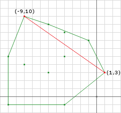
Now, if we say that Q is the closest point to the origin on the termination simplex, then we know that the vector from Q to the origin must be perpendicular to the segment that Q lies on.
L = A – B
Q · L = 0
If we substitute for Q we obtain:
(λ1A + λ2B) · L = 0
We need to solve for λ1 and λ2 but to do so we need 2 equations. The second equation comes from the other part of the definition of a convex hull:
λ1 + λ2 = 1
Solving the system of equations we obtain:
λ2 = -L · A / (L · L)
λ1 = 1 – λ2
If we perform this computation on our example above, we get:
L = (-4, -1) - (1, 3) = (-5, -4)
LdotL = 25 + 16 = 41
LdotA = -5 - 12 = -17
λ2 = 17/41
λ1 = 24/41
After computing λ1 and λ2 we can compute the closest points by using the definition of the convex hull again, but using the points that made up the Minkowski Difference points:
Aclosest = λ1As1 + λ2Bs1
Bclosest = λ1As2 + λ2Bs2

Aclosest = 24/41 * (9, 9) + 17/41 * (4, 5) ≈ (6.93, 7.34)
Bclosest = 24/41 * (8, 6) + 17/41 * (8, 6) = (8, 6)
As we can see we computed the closest points!
There are a couple of problems here we must resolve however.
First, if the Minkowski Difference points A and B are the same point, then L will be the zero vector. This means that later when we divide by the magnitude of L we will divide by zero: not good. What this means is that the closest point to the origin is not on a edge of the Minkowski Difference but is a point. Because of this, the support points that made both A and B are the same, and therefore you can just return the support points of A or B:
if (L.isZero()) {
  Aclosest = A.s1;
  Bclosest = A.s2;
}
The second problem comes in when either λ1 or λ2 is negative. According to the definition of a convex hull, λ must be greater than zero. If λ is negative, this tells us that the support points of the other Minkowski Difference point are the closest points:
if (lambda1 < 0) {
  Aclosest = B.s1;
  Bclosest = B.s2;
} else if (lambda2 < 0) {
  Aclosest = A.s1;
  Bclosest = A.s2;
}
Although your tuturial was very helpful and easy to follow, I found some issues:
- On the first iteration, you picked ‘p’ as (1, 3), when the
calculation yelds (1.7, 2.51).
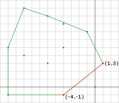
- In the situation shown on fig1.jpg the minkowski difference (blue dots)
doesn’t contain the origin(white dot), but still, the closestPointToOrigin()
routine returns (0,0);
To fix that, before the return i put the following statements:
if the found point is between a and b
return it
else if a.magnitude() < b.magnitude()
return a
else
return b
And the result is fig2.jpg, note that p is the same as a.
F.Y.I: the squares are 20×20 pixels.
Could you give me a opinion about that?
Thank you!
–
fig1.jpg :
fig2.jpg :
Rodrigo,
Sorry for the late response. Now I just to remember how this works….
To answer the first question: You are right that (1.7, 2.51) is the closest point if the simplex was a line, since it isn’t, the closest point is the end point of the line segment. Now I haven’t fully thought it through yet, but it may not matter because you still obtain a vector in that points to the same Voronoi region of the simplex. Ideally, I think you would want d to always be the simplex normal in the direction of the origin.
The second question is bit tricky: What you have found here is a degenerate case! If you look closely, the origin actually lies on the line created by the simplex points, thereby causing the result to be zero. Even if you do something like what I suggested in the first questions answer, this can still happen depending on the method you arrive at the closest point. So in this case, you do have to do something different, which is keep the points who are closest to the origin (so you must pick 2 of the 3). What you have suggested is similar to what I do as well.
In iteration 3, after finding the new direction d(0.62, -0.78), then the point in that direction should be (-4,-1). It is the same with the point added in the iteration 2. My reason is (-4,-1) dot (0.62,-0.78)=-1.7. It is larger than the dot product of (1,3) and (0.62,-0.78)=-1.72. Would you please tell me why you choose (1,3) here? Thanks very much.
The other point could have been chosen as well. If we use better precision than in the examples above the choice to use the point (9, 9) or (4, 5) becomes apparent:
d.dot(4, 5) = -1.405563856997454589716925831015
d.dot(9, 9) = -1.405563856997454589716925831017
You’ll notice that (9, 9) is insignificantly smaller than (4, 5) and if in your code you use floating point variables, they will be identical. This is the case because the direction vector is the normal of the edge (9, 9) to (4, 5) and therefore the projection of both points should be the same.
In these cases, you can use either one, it doesn’t matter, you’ll get the same result!
I notice that in this post, you first find the new point P = AB.mult(t).add(A), then the search in the direction of -P. While in the previous post, the direction is found by doing the triple cross product. What’s the reason for this? Thanks.
I’m trying to use this case to see how to jump out of the loop. Starting with A(1,3) and B(-9,10), then doing triple cross product ABxAOxAB give the direction (-0.573,-0.819). Then I use all the vertices on the edge to dot product with the direction vector. For 3 vertices give positive values and vertex (-11,-1) gives the largest one (Question 1: Here, should I check if the simplex contains the origin?).
So (-11,-1) is added on as the new point A, same as in your post. Then I do the triple cross product to find the direction (0.316, -0.949) to search. doing dot product of all vertices with the new searching direction gives all negative values. So, question 2, does it mean the loop should be terminated here? or should I keep on searching in another direction until it leads back to the vertex that has already been checked before? Cuz when I keep on doing triple cross product to find the new point, it leads me to (-4,-1), and then back to (1,3) where I started.
Thanks a lot for answering all my questions.
That’s a good observation. The reason they are done differently is because of the assumptions. In the first post we are making the assumption that the origin lies within the Minkowski sum, terminating when we verify this (or cannot verify). Because we need to know where the origin lies (by voronoi regions) and find a new search direction, we just put the two together.
Finding the distance is similar but slightly different. No longer are we checking if the simplex contains the origin since the assumption is that the Minkowski sum does not contain the origin. In addition, the simplex is a line segment, instead of a triangle, and therefore cannot contain the origin (if we ignore cases where the origin is on the line segment). Because of this we don’t need to worry about voronoi regions or where the origin lies. The search direction is always the normal of the line segment in the direction of the origin.
Given that, I chose to use P = AB.mult(t).add(A) which obtains the point on the line segment that is closest to the origin so that when the loop terminates I’ll be able to get the separation distance by simply getting the magnitude of P.
No problem, these questions will help everyone who reads them.
As for question 1: You do not have to check if the simplex contains the origin. The simplex in the distance check is a line segment anyway and can only “contain” the origin if the origin lies on the line segment, in which case you must determine if this is considered a collision or not. You may have noticed that in my code I do check if the origin lies within the triangle (before throwing away one of the points). I do this because my distance method can be called by anyone, and they may not know that the distance method assumes that the shapes are separated. Otherwise I would remove that check.
As for question 2: Right, the termination case is a bit tricky. You know to terminate the loop when the new point you found via the support function is projected onto the search direction and that projection is not greater than zero.
So in iteration 1, you find c, the new point, to be (-11, -1). If we project this onto the search direction:
d.dot(-11, -1) = -0.32 * -11 + -0.95 * -1 = 4.47
It’s greater than zero so that means that we were able to move the simplex in the given direction.
So in iteration 2, you find c to be (-4, -1). If we project this onto the search direction:
d.dot(-4, -1) = 0.32 * -4 + -0.95 * -1 = 0.15
It’s greater than zero so that means that we were able to move the simplex in the given direction.
Now in iteration 3, you find c to be (1, 3) or (-4, -1). If we project this onto the search direction:
d.dot(1, 3) = 0.62 * 1 + -0.78 * 3 = -1.72 or
d.dot(-4, -1) = 0.62 * -4 + -0.78 * -1 = -1.7
Here we see that the projection of the point(s) is less than zero, this means that we cannot get any closer to the origin.
So right now my understanding is:
If we have two objects in interaction, then we’ll always be able to locate at least one point giving a positive dot product in the direction we’re searching for. And for each point added in, we can generate a simplex to determine if it contains the origin. And eventually we’ll find such origin.
If the two objects are not in contact, we’ll soon jump out of the loop when we can not find any points giving positive “dot product”.
Is it correct?
One more question, I’m trying to do a 3D case. So I need to build a triangle first then add a point in the search direction to get a tetrahedron. How to get the first triangle? With the same method in 2D, I can easily find a line segment, then doing a triple cross product will give a third point and thus generating a triangle. Do you think this can be the triangle to start with? thanks.
Yes, you are correct.
For the 3D case you can build a triangle (after building the line segment) by obtaining a normal of the line segment in the direction of the origin:
Now that you have a triangle your next search direction would be the surface normal of the triangle in the direction of the origin. Then obtain a support point, then reduce the 4 points to 3.
Hi William,
First of all, thanks for the great articles you’ve put online!
I’ve been playing with an implementation in C#/WPF based on this text and the dyn4j code. Everything looks quite alright but there is an small issue with the closest point that you might be able to give me some hints on.
I have the following (default) quadrant setup;
4 | 1
——–
3 | 2
the origin (0,0) is in the middle of my screen. q1 = x > 0 && y > 0; q2 = x > 0 && y < 0 and so on.
The results look fine whenever I keep both polygons inside the first quadrant. i.e. all the vertices have a positive value. As soon as I move one or more shapes to a different region the closest points start to drift. Is this something you've seen before using this algorithm or am I overlooking a minus sign somewhere and just need to look harder?
Thanks!
Ernst
b.t.w. I'm in 2d as you might have guessed.
No I haven’t seen that behavior before. What do you mean by drift?
The first thing I would check is if the distance check is working correctly minus the closest points in all quadrants. Then I would make sure that the Minkowski points are correct. The Minkowski points should be the points on the Minkowski sum that form the edge that is closest to the origin (see Figure 6).
If you still can’t find the problem you are welcome to send me the code via or by posting it here.
William
Thanks for your reply! By drifting I mean that the points leave the polygon and lag behind if you move the polygon around. It’s perhaps a bit difficult to explain in text but it looks as if the closest points have a smaller radius of action.
That’s a good suggestion and thanks for your offer. I’ll check if the points fall onto the sum shape. Maybe there is an error I can spot.
I’ll let you know!
thanks,
Ernst
right…. it looks like this was a drawing error and not an algorithmic one!
I was using the Margin property of an Ellipse to define it’s offset from the borders.
This works as long as positive integral values are provided. Negative, non-integral values for margin values are technically permitted, but should be avoided because they are rounded by the layout rounding behavior.
This perfectly explains the behavior I was seeing where points would ‘lag behind’ a shape.
Again, thanks for you suggestions. It helped me verify the points where chosen correctly but just drawn incorrectly.
On to the EPA article :)
cheers!
Ernst