The next equality constraint we will derive is the distance constraint. A distance constraint can be used to join two bodies at a fixed distance. It can also be used as a spring between two bodies.

1. Problem Definition
2. Process Overview
3. Position Constraint
4. The Derivative
5. Isolate The Velocities
6. Compute The K Matrix

Problem Definition
It’s probably good to start with a good definition of what we are trying to accomplish.

We want to take two or more bodies and constrain their motion in some way. For instance, say we want two bodies to only be able to rotate about a common point (Revolute Joint). The most common application are constraints between pairs of bodies. Because we have constrained the motion of the bodies, we must find the correct velocities, so that constraints are satisfied otherwise the integrator would allow the bodies to move forward along their current paths. To do this we need to create equations that allow us to solve for the velocities.

What follows is the derivation of the equations needed to solve for a Distance constraint.

Process Overview
Let’s review the process:

1. Create a position constraint equation.
2. Perform the derivative with respect to time to obtain the velocity constraint.
3. Isolate the velocity.

Using these steps we can ensure that we get the correct velocity constraint. After isolating the velocity we inspect the equation to find J, the Jacobian.

Most constraint solvers today solve on the velocity level. Earlier work solved on the acceleration level.

Once the Jacobian is found we use that to compute the K matrix. The K matrix is the A in the Ax = b general form equation.

Position Constraint
So the first step is to write out an equation that describes the constraint. A Distance Joint should allow the two bodies to move and rotate freely, but should keep them at a certain distance from one another. In other words:

which says that the current distance, and the desired distance, must be equal to zero.

The Derivative
The next step after defining the position constraint is to perform the derivative with respect to time. This will yield us the velocity constraint.

The velocity constraint can be found/identified directly, however its encouraged that a position constraint be created first and a derivative be performed to ensure that the velocity constraint is correct.

Another reason to write out the position constraint is because it can be useful during whats called the position correction step; the step to correct position errors (drift).

First if we write out how is computed we obtain:

Where and are the anchor points on the respective bodies.

We can rewrite this equation changing the magnitude to:

Since the squared magnitude of a vector is the dot product of the vector and itself.

Now we perform the derivative:

First let:

so

by the chain rule:

by the chain rule again:

Since the dot product is cumulative and distributive over addition:

If we clean up a bit:

Now we know that:

The derivative of a fixed length vector under a rotation frame is the cross product of the angular velocity with that fixed length vector.

So

We can also let:

Giving us:

Isolate The Velocities
The next step involves isolating the velocities and identifying the Jacobian. This may be confusing at first because there are two velocity variables. In fact, there are actually four, the linear and angular velocities of both bodies. To isolate the velocities we will need to employ some identities and matrix math.

The linear velocities are already isolated so we can ignore those for now. The angular velocities on the other hand have a pesky cross product. In 3D, we can use the identity that a cross product of two vectors is the same as the multiplication by a skew symmetric matrix and the other vector; see . For 2D, we can do something similar by examining the cross product itself:

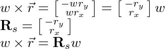
Remember that the angular velocity in 2D is a scalar.

Removing the cross products using the process above yields:

Now if we employ some matrix multiplication we can separate the velocities from the known coefficients:

Now, by inspection, we obtain the Jacobian:

Compute The K Matrix
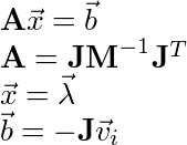
Lastly, to solve the constraint we need to compute the values for A (I use the name K) and b:

See the “Equality Constraints” post for the derivation of the A matrix and b vector.

The b vector is fairly straight forward to compute. Therefore I’ll skip that and compute the K matrix symbolically:

Multiplying left to right the first two matrices we obtain:

Multiplying left to right again:

Multiplying left to right again:

Finally distributing the last term and pulling out scalar values we get:

Remember the inertia tensor in 2D is a scalar, therefore we can pull it out to the front of the multiplications.

Since n is normalized:

We get:

Then if we perform the matrix multiplication in the other terms:

We obtain (remember the cross product in 2D is a scalar):

Plug the values of the K matrix and b vector into your linear equation solver and you will get the impulse required to satisfy the constraint.

Note here that if you are using an iterative solver that the K matrix does not change over iterations and as such can be computed once each time step.

Another interesting thing to note is that the K matrix will always be a square matrix with a size equal to the number of degrees of freedom (DOF) removed. This is a good way to check that the derivation was performed correctly.