Code Zealot » Constrained Dynamics

Prismatic Constraint

Sat, 12 Mar 2011 23:52:03 +0000

The next equality constraint we will derive is the prismatic constraint. A prismatic constraint is like the line constraint except it does not allow rotation about the anchor point. A prismatic constraint constraints the linear motion of the bodies along a line. An example of a prismatic joint is the slide of a semi-automatic pistol. The slide is moved back to charge the weapon, then released to its original position. The slide cannot rotate about the pistol, nor can it move up/down or left/right only along one axis.

Problem Definition
Process Overview
The Jacobian
Compute The K Matrix

Problem Definition
It’s probably good to start with a good definition of what we are trying to accomplish.

We want to take two or more bodies and constrain their motion in some way. For instance, say we want two bodies to only be able to rotate about a common point (Revolute Joint). The most common application are constraints between pairs of bodies. Because we have constrained the motion of the bodies, we must find the correct velocities, so that constraints are satisfied otherwise the integrator would allow the bodies to move forward along their current paths. To do this we need to create equations that allow us to solve for the velocities.

What follows is the derivation of the equations needed to solve for a Prismatic constraint.

Process Overview
Let’s review the process:

Create a position constraint equation.
Perform the derivative with respect to time to obtain the velocity constraint.
Isolate the velocity.

Using these steps we can ensure that we get the correct velocity constraint. After isolating the velocity we inspect the equation to find J, the Jacobian.

Most constraint solvers today solve on the velocity level. Earlier work solved on the acceleration level.

Once the Jacobian is found we use that to compute the K matrix. The K matrix is the A in the Ax = b general form equation.

The Jacobian
As earlier stated, the Prismatic Joint is just like the Line Joint only it does not allow rotation about the anchor point. Because of this, we can formulate the Prismatic Joint by combining two joints: Line Joint and Angle Joint. This allows us to skip directly to the Jacobian:

See the “Line Constraint” and “Angle Constraint” posts for the derivation of their Jacobians.

Compute The K Matrix
Lastly, to solve the constraint we need to compute the values for A (I use the name K) and b:

See the “Equality Constraints” post for the derivation of the A matrix and b vector.

The b vector is fairly straight forward to compute. Therefore I’ll skip that and compute the K matrix symbolically:

Multiplying left to right the first two matrices we obtain:

Multiplying left to right again:

If we use the following just to clean things up:

We get:

And if t is normalized we get:

Plug the values of the K matrix and b vector into your linear equation solver and you will get the impulse required to satisfy the constraint.

Note here that if you are using an iterative solver that the K matrix does not change over iterations and as such can be computed once each time step.

Another interesting thing to note is that the K matrix will always be a square matrix with a size equal to the number of degrees of freedom (DOF) removed. This is a good way to check that the derivation was performed correctly.

]]>

Line Constraint

Fri, 31 Dec 2010 01:45:04 +0000

The next equality constraint we will derive is the line constraint. A line constraint is like a prismatic constraint (which will most likely be the next post) except allows rotation about the anchor point. A prismatic constraint constraints the linear motion of the bodies along a line. An example of a prismatic joint might be a roller coaster on the track. The cars cannot translate or rotate except along the track. For simplicity the prismatic constraint we will define is only for straight lines.

Problem Definition
Process Overview
Position Constraint
The Derivative
Isolate The Velocities
Compute The K Matrix

Problem Definition
It’s probably good to start with a good definition of what we are trying to accomplish.

What follows is the derivation of the equations needed to solve for a Line constraint.

Process Overview
Let’s review the process:

Create a position constraint equation.
Perform the derivative with respect to time to obtain the velocity constraint.
Isolate the velocity.

Using these steps we can ensure that we get the correct velocity constraint. After isolating the velocity we inspect the equation to find J, the Jacobian.

Most constraint solvers today solve on the velocity level. Earlier work solved on the acceleration level.

where:

If we examine the equation we can see that this will allow us to constraint the linear motion. This equation states that any motion that is not along the vector u is invalid, because the tangent of that motion projected onto (via the dot product) the u vector will no longer yield 0.

The initial vector u will be supplied in the construction of the constraint. From u, we will obtain the tangent of u, the t vector. Each simulation step we will recompute u from the anchor points and use it along with the saved t vector to determine if the constraint has been violated.

Notice that this does not constrain the rotation of the bodies about the anchor point however. To also constrain the rotation about the anchor point use a prismatic joint.

The Derivative
The next step after defining the position constraint is to perform the derivative with respect to time. This will yield us the velocity constraint.

The velocity constraint can be found/identified directly, however its encouraged that a position constraint be created first and a derivative be performed to ensure that the velocity constraint is correct.

Another reason to write out the position constraint is because it can be useful during whats called the position correction step; the step to correct position errors (drift).

By the chain rule:

Where the derivative of u:

The derivative of a fixed length vector under a rotation frame is the cross product of the angular velocity with that fixed length vector.

And the derivative of t:

Here is one tricky part about this derivation. We know that t, like r in the u derivation, is a fixed length vector under a rotation frame. A vector can only be fixed in one coordinate frame, therefore you must choose one: a or b. I chose b, but either way, as long as the K matrix and b vector derivations are correct it will still solve the constraint.

Substituting these back into the equation creates:

Now we need to distribute, and on the last term I’m going to use the property that dot products are commutative:

Now we need to group like terms, but the terms are jumbled. We can use the identity:

and the property that dot products are commutative to obtain:

Now we can use the property that the cross product is anti-commutative on the last term to obtain the following. Then we group by like terms:

Isolate The Velocities
The next step involves isolating the velocities and identifying the Jacobian. This may be confusing at first because there are two velocity variables. In fact, there are actually four, the linear and angular velocities of both bodies. To isolate the velocities we will need to employ some identities and matrix math.

All the velocity terms are already ready to be isolated, by employing some matrix math we can obtain:

By inspection the Jacobian is:

Compute The K Matrix
Lastly, to solve the constraint we need to compute the values for A (I use the name K) and b:

See the “Equality Constraints” post for the derivation of the A matrix and b vector.

The b vector is fairly straight forward to compute. Therefore I’ll skip that and compute the K matrix symbolically:

Multiplying left to right the first two matrices we obtain:

Multiplying left to right again:

Plug the values of the K matrix and b vector into your linear equation solver and you will get the impulse required to satisfy the constraint.

Note here that if you are using an iterative solver that the K matrix does not change over iterations and as such can be computed once each time step.

]]>

Weld Constraint

Thu, 30 Dec 2010 22:05:41 +0000

The next equality constraint we will derive is the weld constraint. A weld constraint can be used to join two bodies at an anchor point in which the bodies must move and rotate together (all DOF are constrained).

This post will differ slightly from the previous posts. A weld joint is basically a revolute joint + an angle joint. In that case we can use the resulting Jacobians from those posts to skip a bit of the work.

Problem Definition
Process Overview
The Jacobian
Compute The K Matrix

Problem Definition
It’s probably good to start with a good definition of what we are trying to accomplish.

What follows is the derivation of the equations needed to solve for a Weld constraint.

Process Overview
Let’s review the process:

Create a position constraint equation.
Perform the derivative with respect to time to obtain the velocity constraint.
Isolate the velocity.

Using these steps we can ensure that we get the correct velocity constraint. After isolating the velocity we inspect the equation to find J, the Jacobian.

Most constraint solvers today solve on the velocity level. Earlier work solved on the acceleration level.

Once the Jacobian is found we use that to compute the K matrix. The K matrix is the A in the Ax = b general form equation.

The Jacobian
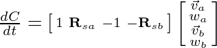
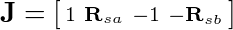
Like stated above, the weld constraint is just a combination of two other constraints: point-to-point and angle constraints. As such, we can simply combine the Jacobians we found for those constraints into one Jacobain:

See the “Point-to-Point Constraint” and “Angle Constraint” posts for the derivation of their Jacobians.

Compute The K Matrix
Lastly, to solve the constraint we need to compute the values for A (I use the name K) and b:

See the “Equality Constraints” post for the derivation of the A matrix and b vector.

For this constraint the b vector computation isn’t as simple as in past constraints. So I’ll work this out as well:

Notice here that the first element in the b vector is a vector also. This makes the b vector a 3×1 vector instead of the normal 2×1 that we have seen thus far.

Now on to computing the K matrix:

Multiplying left to right the first two matrices we obtain:

Multiplying left to right again:

Unlike previous posts, some of the elements in the above matrix are matrices themselves. When we multiply out the elements we’ll see that the resulting K matrix is actually a 3×3 matrix.

It makes sense that the K matrix is a 3×3 because the b vector was a 3×1, meaning we have 3 variables to solve for. The b vector and K matrix dimensions must match.

So lets take each element and work them out separately, starting with the first element. We can actually copy the result from the Point-to-Point constraint post since its exactly the same:

Now let move on to the second element. If we remember:

So multiplying and adding the vectors here yields the matrix:

Likewise, for the third element:

Lastly the last element can be left as is since its just a scalar.

Now adding all these elements back into one big matrix we obtain:

Plug the values of the K matrix and b vector into your linear equation solver and you will get the impulse required to satisfy the constraint.

Note here that if you are using an iterative solver that the K matrix does not change over iterations and as such can be computed once each time step.

]]>

Angle Constraint

Thu, 30 Dec 2010 19:45:25 +0000

The next equality constraint we will derive is the angle constraint. An angle constraint can be used to join two bodies forcing them to have the same rotation. This particular constraint will be added to other constraints (in later posts) to form more complex constraints.

Problem Definition
Process Overview
Position Constraint
The Derivative
Isolate The Velocities
Compute The K Matrix

Problem Definition
It’s probably good to start with a good definition of what we are trying to accomplish.

What follows is the derivation of the equations needed to solve for an Angle constraint.

Process Overview
Let’s review the process:

Create a position constraint equation.
Perform the derivative with respect to time to obtain the velocity constraint.
Isolate the velocity.

Using these steps we can ensure that we get the correct velocity constraint. After isolating the velocity we inspect the equation to find J, the Jacobian.

Most constraint solvers today solve on the velocity level. Earlier work solved on the acceleration level.

which says that the rotation about the center of body a minus the rotation about the center of body b should equal the initial reference angle calculated when the joint was created.

The Derivative
The next step after defining the position constraint is to perform the derivative with respect to time. This will yield us the velocity constraint.

The velocity constraint can be found/identified directly, however its encouraged that a position constraint be created first and a derivative be performed to ensure that the velocity constraint is correct.

Another reason to write out the position constraint is because it can be useful during whats called the position correction step; the step to correct position errors (drift).

As a side note, this is one of the easiest constraints to both derive and implement.

Start by taking the derivative of the position constraint:

Isolate The Velocities
The next step involves isolating the velocities and identifying the Jacobian. This may be confusing at first because there are two angular velocity variables. To isolate the velocities we will need to employ some matrix math.

Notice that I still included the linear velocities in the equation even though they are not present. This is necessary since the mass matrix is a 4×4 matrix so that we can multiply the matrices in the next step.

Now, by inspection, we obtain the Jacobian:

Compute The K Matrix
Lastly, to solve the constraint we need to compute the values for A (I use the name K) and b:

See the “Equality Constraints” post for the derivation of the A matrix and b vector.

The b vector is fairly straight forward to compute. Therefore I’ll skip that and compute the K matrix symbolically:

Multiplying left to right the first two matrices we obtain:

Multiplying left to right again:

Plug the values of the K matrix and b vector into your linear equation solver and you will get the impulse required to satisfy the constraint.

Note here that if you are using an iterative solver that the K matrix does not change over iterations and as such can be computed once each time step.

]]>

Pulley Constraint

Thu, 30 Dec 2010 18:32:42 +0000

The next equality constraint we will derive is the pulley constraint. A pulley constraint can be used to join two bodies at a fixed distance. In addition, the constraint can be used to simulate a block-and-tackle.

Problem Definition
Process Overview
Position Constraint
The Derivative
Isolate The Velocities
Compute The K Matrix

Problem Definition
It’s probably good to start with a good definition of what we are trying to accomplish.

What follows is the derivation of the equations needed to solve for a Pulleyconstraint.

Process Overview
Let’s review the process:

Create a position constraint equation.
Perform the derivative with respect to time to obtain the velocity constraint.
Isolate the velocity.

Using these steps we can ensure that we get the correct velocity constraint. After isolating the velocity we inspect the equation to find J, the Jacobian.

Most constraint solvers today solve on the velocity level. Earlier work solved on the acceleration level.

Once the Jacobian is found we use that to compute the K matrix. The K matrix is the A in the Ax = b general form equation.

Position Constraint
So the first step is to write out an equation that describes the constraint. A Distance Joint should allow the two bodies to move and rotate freely, but should keep them at a certain distance from one another. For a Pulley Joint its similar except that the bodes distance is constrained to two axes. In the middle we will allow the option of a block-and-tackle. Examining the image to the right, we see that there are two bodies: Ba, Bb who have distance constraints that are along axes: Ua, Ub which were formed from the Ground and Body anchor points: GAa, GAb, BAa, BAb.

Given this definition we can see that the direction of Ua and Ub can change if the bodies swing left or right for example.

Unlike the Distance Joint, a Pulley Joint allows the distances from the ground anchors to the body anchors to increase and decrease (the magnitude of Ua and Ub can also change). However, the total distance along the two axes must be equal to the initial distance when the joint was created (this is what we are trying to constrain). If we apply some scalar factor (or ratio) to the distances we can simulate a block-and-tackle.

We can represent this constraint by the following equation:

Where:

Where are the length of Ua, body a’s body anchor point, body a’s ground anchor point, and the vector Ua respectively.

Likewise are the length of Ub, body b’s body anchor point, body b’s ground anchor point, and the vector Ub respectively.

is computed once when the joint is created to obtain the target total length of the pulley.

Finally is a scalar ratio value that will allow us to simulate a block-and-tackle.

To review, our position constraint calculates the current lengths of the two axes (applying the ratio to one) and subtracts it from the initial to find how much the constraint is violated.

The Derivative
The next step after defining the position constraint is to perform the derivative with respect to time. This will yield us the velocity constraint.

The velocity constraint can be found/identified directly, however its encouraged that a position constraint be created first and a derivative be performed to ensure that the velocity constraint is correct.

Another reason to write out the position constraint is because it can be useful during whats called the position correction step; the step to correct position errors (drift).

Taking the derivative of our position constraint we get:

Then just to clean up a bit:

Now we need to perform the derivative on . If we remember was defined as:

So let’s side step for a minute and perform the derivative of :

We needed to use the chain rule in order to fully compute the derivative where the derivative of u:

The derivative of a fixed length vector under a rotation frame is the cross product of the angular velocity with that fixed length vector.

Note here that the g vector (ground anchor) is constant and therefore becomes the zero vector.

In the last few steps I replaced a portion of the equation with:

In addition, I replaced the dot product with a matrix multiplication by:

Now if we substitute back into the original equation we get:

The linear velocities are already isolated so we can ignore those for now. The angular velocities on the other hand have a pesky cross product. In 3D, we can use the identity that a cross product of two vectors is the same as the multiplication by a skew symmetric matrix and the other vector; see . For 2D, we can do something similar by examining the cross product itself:

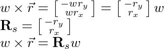
Remember that the angular velocity in 2D is a scalar.

Removing the cross products using the process above yields:

Now, just to clean up some, if we inspect:

Now replacing what we found above into the original equation (and some clean up):

Now if we employ some matrix multiplication we can separate the velocities from the known coefficients:

Now, by inspection, we obtain the Jacobian:

Compute The K Matrix
Lastly, to solve the constraint we need to compute the values for A (I use the name K) and b:

See the “Equality Constraints” post for the derivation of the A matrix and b vector.

The b vector is fairly straight forward to compute. Therefore I’ll skip that and compute the K matrix symbolically:

Multiplying left to right the first two matrices we obtain:

Multiplying left to right again:

If we simplify using:

Remember the inertia tensor in 2D is a scalar, therefore we can pull it out to the front of the multiplications.

Plug the values of the K matrix and b vector into your linear equation solver and you will get the impulse required to satisfy the constraint.

Note here that if you are using an iterative solver that the K matrix does not change over iterations and as such can be computed once each time step.

]]>

Max Distance Constraint

Sat, 18 Dec 2010 18:22:59 +0000

As a follow up post to the Distance Constraint post, we can also create a maximum distance constraint using the same solution we found in the Distance Constraint post.

The previous solution created a fixed length distance constraint which forced a pair of bodies to be a given length apart. We can simply add an if statement to make this constraint a max length constraint.

A max length constraint only specifies that the distance between the joined bodies does not exceed the given maximum. So before applying the fixed length distance constraint just check whether the bodies have separated past the maximum distance. If not, then do nothing. Simple!

l = (pa - pb).getMagnitude();
if (l > maxDistance) {
  // apply constraint
}
// otherwise do nothing

]]>

Distance Constraint

Sat, 11 Sep 2010 18:07:48 +0000

The next equality constraint we will derive is the distance constraint. A distance constraint can be used to join two bodies at a fixed distance. It can also be used as a spring between two bodies.

Problem Definition
Process Overview
Position Constraint
The Derivative
Isolate The Velocities
Compute The K Matrix

Problem Definition
It’s probably good to start with a good definition of what we are trying to accomplish.

What follows is the derivation of the equations needed to solve for a Distance constraint.

Process Overview
Let’s review the process:

Create a position constraint equation.
Perform the derivative with respect to time to obtain the velocity constraint.
Isolate the velocity.

Using these steps we can ensure that we get the correct velocity constraint. After isolating the velocity we inspect the equation to find J, the Jacobian.

Most constraint solvers today solve on the velocity level. Earlier work solved on the acceleration level.

which says that the current distance, and the desired distance, must be equal to zero.

The Derivative
The next step after defining the position constraint is to perform the derivative with respect to time. This will yield us the velocity constraint.

The velocity constraint can be found/identified directly, however its encouraged that a position constraint be created first and a derivative be performed to ensure that the velocity constraint is correct.

Another reason to write out the position constraint is because it can be useful during whats called the position correction step; the step to correct position errors (drift).

First if we write out how is computed we obtain:

Where and are the anchor points on the respective bodies.

We can rewrite this equation changing the magnitude to:

Since the squared magnitude of a vector is the dot product of the vector and itself.

Now we perform the derivative:

First let:

by the chain rule:

by the chain rule again:

Since the dot product is cumulative and distributive over addition:

If we clean up a bit:

Now we know that:

The derivative of a fixed length vector under a rotation frame is the cross product of the angular velocity with that fixed length vector.

We can also let:

Giving us:

Remember that the angular velocity in 2D is a scalar.

Removing the cross products using the process above yields:

Now if we employ some matrix multiplication we can separate the velocities from the known coefficients:

Now, by inspection, we obtain the Jacobian:

Compute The K Matrix
Lastly, to solve the constraint we need to compute the values for A (I use the name K) and b:

See the “Equality Constraints” post for the derivation of the A matrix and b vector.

The b vector is fairly straight forward to compute. Therefore I’ll skip that and compute the K matrix symbolically:

Multiplying left to right the first two matrices we obtain:

Multiplying left to right again:

Finally distributing the last term and pulling out scalar values we get:

Remember the inertia tensor in 2D is a scalar, therefore we can pull it out to the front of the multiplications.

Since n is normalized:

We get:

Then if we perform the matrix multiplication in the other terms:

We obtain (remember the cross product in 2D is a scalar):

Plug the values of the K matrix and b vector into your linear equation solver and you will get the impulse required to satisfy the constraint.

Note here that if you are using an iterative solver that the K matrix does not change over iterations and as such can be computed once each time step.

]]>

Point-to-Point Constraint

Sun, 25 Jul 2010 02:47:38 +0000

As the first entry after the Equality Constraints post, we will perform the derivation of the Point-to-Point constraint, which models a Revolute Joint, in 2D.

Problem Definition
Process Overview
Position Constraint
The Derivative
Isolate The Velocities
Compute The K Matrix

Problem Definition
It’s probably good to start with a good definition of what we are trying to accomplish. From the last post on equality constraints it may not be clear what we are trying to do.

What follows is the derivation of the equations needed to solve for a Point-to-Point constraint which models a Revolute Joint.

Process Overview
Since this is the first specific constraint I’ll post on, we need to go through how we actually perform the derivation.

lays out the process quite simply:

Create a position constraint equation.
Perform the derivative with respect to time to obtain the velocity constraint.
Isolate the velocity.

Using this formula we can ensure that we get the correct velocity constraint. After isolating the velocity we inspect the equation to find J, the Jacobian.

Most constraint solvers today solve on the velocity level. Earlier work solved on the acceleration level.

which says the points and must be the same point. This allows the bodies to translate freely but only together.

The Derivative
The next step after defining the position constraint is to perform the derivative with respect to time. This will yield us the velocity constraint.

The velocity constraint can be found/identified directly, however its encouraged that a position constraint be created first and a derivative be performed to ensure that the velocity constraint is correct.

Another reason to write out the position constraint is because it can be useful during whats called the position correction step; the step to correct position errors (drift).

First if we write out how and are computed we obtain:

Where and are the centers of mass (or positions), and are the rotation matrices, and and are the vectors from the centers of mass to the common point.

Now that the constraint is written in the correct variables we can perform the derivative:

The derivative of a fixed length vector under a rotation frame is the cross product of the angular velocity with that fixed length vector.

Remember that the angular velocity in 2D is a scalar.

Removing the cross products using the process above yields:

Now if we employ some matrix multiplication we can separate the velocities from the known coefficients:

Now, by inspection, we obtain the Jacobian:

Compute The K Matrix
Lastly, to solve the constraint we need to compute the values for A (I use the name K) and b:

See the “Equality Constraints” post for the derivation of the A matrix and b vector.

The b vector is fairly straight forward to compute. Therefore I’ll skip that and compute the K matrix symbolically:

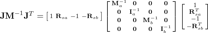
Multiplying left to right the first two matrices we obtain:

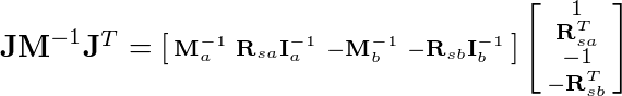
Multiplying left to right again:

Now if we write out the equation element wise:

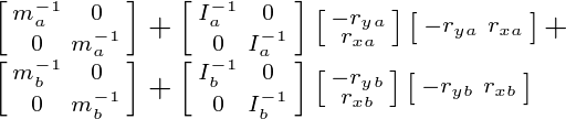
Remember the inertia tensor in 2D is a scalar, therefore we can pull it out to the front of the multiplications.

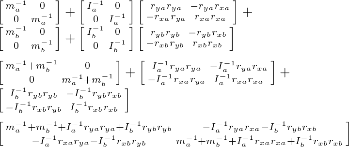
Multiplying the matrices and adding them yields:

Plug the values of the K matrix and b vector into your linear equation solver and you will get the impulse required to satisfy the constraint.

Note here that if you are using an iterative solver that the K matrix does not change over iterations and as such can be computed once each time step.

]]>

Equality Constraints

Sat, 24 Jul 2010 18:36:21 +0000

After the first release of the project, I felt that it would be good to pass along what I learned about constrained dynamics.

This is not an easy subject and aside from purchasing books there’s not much information out there about it for those of us not accustomed to reading research papers or theses.

In this post I plan to solve a velocity constraint generally. Later posts will be for the individual types of constraints.

A phyiscial constraint is defined by some function:

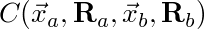
Where x is the position of the body and R is the rotation of the body. Typically constraints are pairwise. You can formulate constraints using any number of bodies, however, pairwise formulations are simple. When this function is equal to zero the constraint is satisfied.

If we perform the derivative with respect to time we get the velocity constraint

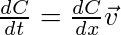
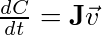
Since C is a function of positions and rotations who are themselves functions of time, we must perform the chain rule. The derivative of one vector function (C) by another vector function (x) yields a Jacobian matrix:

[1]

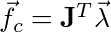
Where v is the vector of velocities from the bodies. The Jacobian rows contain the gradients of the scalar components of the constraint function C. We know that the gradient direction is the highest rate of increase of the scalar function C and unless the constraint is satisfied then it will be non-zero. Therefore the gradient is the direction of the illegal movement. We want the constraint force to act in this direction since we don’t want to constrain legal movement:

[2]

Where lambda a vector of the magnitudes of the constraint forces. The constraint force is the force that must be applied to counter act external forces so that the constraint is satisfied.

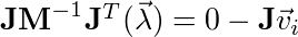
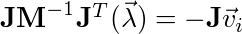
We know that the final velocity of a system is:

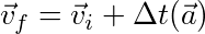
We also know that the sum of all the forces on a body is:

We can split the external forces and the constraint forces apart and then distribute:

If we look closely we can perform the integration using the external forces separately therefore removing the external forces from the equation:

[3]

Now if we substitute equation [2] into [3]:

[4]

Now if we substitue equation [4] into equation [1]:

[5]

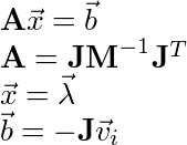
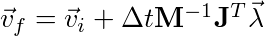
Now if we rearrange the terms to match the form Ax = b:

We also know that:

Where P is the impulse, therefore:

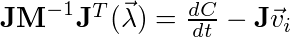[6]

Where lambda is the constraint impulse. We stated at the beginning of the post that if the constraint is satisfied if the constraint equals zero. This is true for the velocity constraint as well:

This will solve the constraint exactly, however, given that the integrator is only an approximation of the ODE and the lack of infinite precision the constraint will “drift.” For example, a point-to-point constraint (simulates a revolute joint) will drift, where the local points of the world space anchor point slowly separate over time.

Drift can be solve using methods like Baumgarte stabilization, post/pre stabilizations methods, etc. That will be left for another post.

The equation is now in the form:

and can be solved using any linear equation solver desired. After solving for lamda, we can substitute it back into equation 4:

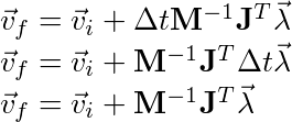
to find the final velocities.

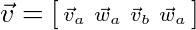
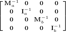
Remember that the velocity vector is the velocity of the system and the mass matrix is the mass of the system. For example, a two body system would have the form:

The Jacobian, as we will see in the next few posts, will be specific to the type of constraint being added and the number of bodies involved (as we see above).

]]>