Of course I’m a bit biased since I was privileged to write the chapter Collision Detection Using the GJK Algorithm (chapter 11). The chapter is about 35 pages long and covers a 2D implementation and explanation of GJK and related algorithms.

Throughout the chapter I explain the concepts with concrete examples and pseudo code. At the end of the last three sections I talk about the robustness of each, focusing on floating point problems and special cases.

Here’s a breif summary of the topics covered in the GJK chapter:

• Introduction to Collision Detection
• Convexity
• Minkwoski Sum
• SAT-GJK (GJK w/o the distance sub algo.)
• GJK Distance and Closest Points
• EPA

Big thanks to the editors of the book for allowing me this great opportunity and an even bigger thanks to my Savior Jesus Christ.

1. Introduction
2. Finding the Features
3. Clipping
4. Example 1
5. Example 2
6. Example 3
7. Curved Shapes
8. Alternative Methods

Introduction
Most collision detection algorithms will return a separation normal and depth. Using this information we can translate the shapes directly to resolve the collision. Doing so does not exhibit real world physical behavior. As such, this isn’t sufficent for applications that want to model the physical world. To model real world iteractions effectively, we need to know where the collision occurred.

Contact points are usually world space points on the colliding shapes/bodies that represent where the collision is taking place. In the real world this would on the edge of two objects where they are touching. However, most simulations run collision detection routines on some interval allowing the objects overlap rather than touch. In this very common scenario, we must infer what the contact(s) should be.

More than one contact point is typically called a contact manifold or contact patch.

Finding the Features
The first step is to identify the features of the shapes that are involved in the collision. We can find the collision feature of a shape by finding the farthest vertex in the shape. Then, we look at the adjacent two vertices to determine which edge is the “closest.” We determine the closest as the edge who is most perpendicular to the separation normal.

// step 1
// find the farthest vertex in
// the polygon along the separation normal
int c = vertices.length;
for (int i = 0; i < c; i++) {
  double projection = n.dot(v);
  if (projection > max) {
    max = projection;
    index = i;
  }
}

// step 2
// now we need to use the edge that
// is most perpendicular, either the
// right or the left
Vector2 v = vertices[index];
Vector2 v1 = v.next;
Vector2 v0 = v.prev;
// v1 to v
Vector2 l = v - v1;
// v0 to v
Vector2 r = v - v0;
// the edge that is most perpendicular
// to n will have a dot product closer to zero
if (r.dot(n) <= l.dot(n)) {
  // the right edge is better
  // make sure to retain the winding direction
  return new Edge(v, v0, v);
} else {
  // the left edge is better
  // make sure to retain the winding direction
  return new Edge(v, v, v1);
}
// we return the maximum projection vertex (v)
// and the edge points making the best edge (v and either v0 or v1)

Be careful when computing the left and right (l and r in the code above) vectors as they both must point towards the maximum point. If one doesn’t that edge may always be used since its pointing in the negative direction and the other is pointing in the positive direction.

To obtain the correct feature we must know the direction of the separation normal ahead of time. Does it point from A to B or does it point from B to A? Its recommended that this is fixed, so for this post we will assume that the separation normal always points from A to B.

// find the "best" edge for shape A
Edge e1 = A.best(n);
// find the "best" edge for shape B
Edge e2 = B.best(-n);

Clipping
Now that we have the two edges involved in the collision, we can do a series of line/plane clips to get the contact manifold (all the contact points). To do so we need to identify the reference edge and incident edge. The reference edge is the edge most perpendicular to the separation normal. The reference edge will be used to clip the incident edge vertices to generate the contact manifold.

Edge ref, inc;
boolean flip = false;
if (e1.dot(n) <= e2.dot(n)) {
  ref = e1;
  inc = e2;
} else {
  ref = e2;
  inc = e1;
  // we need to set a flag indicating that the reference
  // and incident edge were flipped so that when we do the final
  // clip operation, we use the right edge normal
  flip = true;
}

Now that we have identified the reference and incident edges we can begin clipping points. First we need to clip the incident edge’s points by the first vertex in the reference edge. This is done by comparing the offset of the first vertex along the reference vector with the incident edge’s offsets. Afterwards, the result of the previous clipping operation on the incident edge is clipped again using the second vertex of the reference edge. Finally, we check if the remaining points are past the reference edge along the reference edge’s normal. In all, we perform three clipping operations.

ref.normalize();

double o1 = ref.dot(ref.v1);
// clip the incident edge by the first
// vertex of the reference edge
ClippedPoints cp = clip(inc.v1, inc.v2, ref, o1);
// if we dont have 2 points left then fail
if (cp.length < 2) return;

// clip whats left of the incident edge by the
// second vertex of the reference edge
// but we need to clip in the opposite direction
// so we flip the direction and offset
double o2 = ref.dot(ref.v2);
ClippedPoints cp = clip(cp[0], cp[1], -ref, -o2);
// if we dont have 2 points left then fail
if (cp.length < 2) return;

// get the reference edge normal
Vector2 refNorm = ref.cross(-1.0);
// if we had to flip the incident and reference edges
// then we need to flip the reference edge normal to
// clip properly
if (flip) refNorm.negate();
// get the largest depth
double max = refNorm.dot(ref.max);
// make sure the final points are not past this maximum
if (refNorm.dot(cp[0]) - max < 0.0) {
  cp.remove(cp[0]);
}
if (refNorm.dot(cp[1]) - max < 0.0) {
  cp.remove(cp[1]);
}
// return the valid points
return cp;

And the clip method:

// clips the line segment points v1, v2
// if they are past o along n
ClippedPoints clip(v1, v2, n, o) {
  ClippedPoints cp = new ClippedPoints();
  double d1 = n.dot(v1) - o;
  double d2 = n.dot(v2) - o;
  // if either point is past o along n
  // then we can keep the point
  if (d1 >= 0.0) cp.add(v1);
  if (d2 >= 0.0) cp.add(v2);
  // finally we need to check if they
  // are on opposing sides so that we can
  // compute the correct point
  if (d1 * d2 < 0.0) {
    // if they are on different sides of the
    // offset, d1 and d2 will be a (+) * (-)
    // and will yield a (-) and therefore be
    // less than zero
    // get the vector for the edge we are clipping
    Vector2 e = v2 - v1;
    // compute the location along e
    double u = d1 / (d1 - d2);
    e.multiply(u);
    e.add(v1);
    // add the point
    cp.add(e);
  }
}

Even though all the examples use box-box collisions, this method will work for any convex polytopes. See the end of the post for details on handling curved shapes.

Figure 1: A simple box-box collision

Example 1
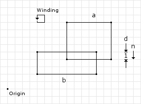
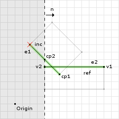
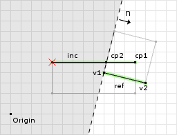
Its best to start with a simple example explaining the process. Figure 1 shows a box vs. box collision with the collision information listed along with the winding direction of the vertices for both shapes. We have following data to begin with:

// from the collision detector
// separation normal and depth
normal = (0, -1)
depth = 1

The first step is to get the “best” edges, or the edges that are involved in the collision:

// the "best" edges    ( max ) | (  v1 ) | ( v2 )
//                    ---------+---------+-------
Edge e1 = A.best(n)  = ( 8, 4) | ( 8, 4) | (14, 4)
Edge e2 = B.best(-n) = (12, 5) | (12, 5) | ( 4, 5)

Figure 2: The “best” edges of figure 1

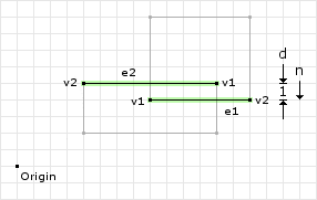
Figure 2 highlights the “best” edges on the shapes. Once we have found the edges, we need to determine which edge is the reference edge and which is the incident edge:

e1 = (8, 4) to (14, 4) = (14, 4) - (8, 4) = (6, 0)
e2 = (12, 5) to (4, 5) = (4, 5) - (12, 5) = (-8, 0)
e1Dotn = (6, 0) ·  (0, -1) = 0
e2Dotn = (-8, 0) · (0, -1) = 0
// since the dot product is the same we can choose either one
// using the first edge as the reference will let this example 
// be slightly simpler
ref = e1;
inc = e2;

Now that we have identified the reference and incident edges we perform the first clipping operation:

ref.normalize() = (1, 0)
o1 = (1, 0) · (8, 4) = 8
// now we call clip with 
// v1 = inc.v1 = (12, 5)
// v2 = inc.v2 = (4, 5)
// n  = ref    = (1, 0)
// o  = o1     = 8
d1 = (1, 0) · (12, 5) - 8 = 4
d2 = (1, 0) · (4, 5)  - 8 = -4
// we only add v1 to the clipped points since
// its the only one that is greater than or
// equal to zero
cp.add(v1);
// since d1 * d2 = -16 we go into the if block
e = (4, 5) - (12, 5) = (-8, 0)
u = 4 / (4 - -4) = 1/2
e * u + v1 = (-8 * 1/2, 0 * 1/2) + (12, 5) = (8, 5)
// then we add this point to the clipped points
cp.add(8, 5);

Figure 3: The first clip of example 1

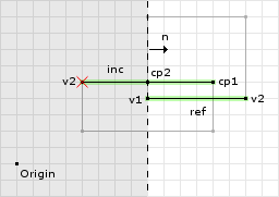
The first clipping operation removed one point that was outside the clipping plane (i.e. past the offset). But since there was another point on the opposite side of the clipping plane, we compute a new point on the edge and use it as the second point of the result. See figure 3 for an illustration.

Since we still have two points in the ClippedPoints object we can continue and perform the second clipping operation:

o2 = (1, 0) · (14, 4) = 14
// now we call clip with
// v1 = cp[0] = (12, 5)
// v2 = cp[1] = (8, 5)
// n  = -ref  = (-1, 0)
// o  = -o1   = -14
d1 = (-1, 0) · (12, 5) - -14 = 2
d2 = (-1, 0) · (8, 5)  - -14 = 6
// since both are greater than or equal
// to zero we add both to the clipped
// points object
cp.add(v1);
cp.add(v2);
// since both are positive then we skip
// the if block and return

Figure 4: The second clip of example 1

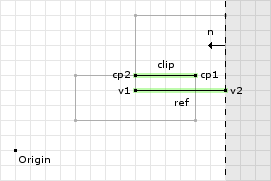
The second clipping operation did not remove any points. Figure 4 shows the clipping plane and the valid and invalid regions. Both points were found to be inside the valid region of the clipping plane. Now we continue to the last clipping operation:

// compute the reference edge's normal
refNorm = (0, 1)
// we didnt have to flip the reference and incident
// edges so refNorm stays the same
// compute the offset for this clipping operation
max = (0, 1) · (8, 4) = 4
// now we clip the points about this clipping plane, where:
// cp[0] = (12, 5)
// cp[1] = (8, 5)
(0, 1) · (12, 5) - 4 = 1
(0, 1) · (8, 5)  - 4 = 1
// since both points are greater than
// or equal to zero we keep them both

Figure 5: The final clip of example 1

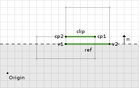
On the final clipping operation we keep both of the points. Figure 5 shows the final clipping operation and the valid region for the points. This ends the clipping operation returning a contact manifold of two points.

// the collision manifold for example 1
cp[0] = (12, 5)
cp[1] = (8, 5)

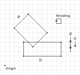
Example 2
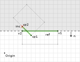
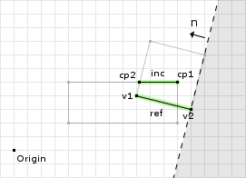
The first example was, by far, the simplest. In this example we will see how the last clipping operation is used. Figure 6 shows two boxes in collision, but in a slightly different configuration. We have following data to begin with:

Figure 6: A more common box-box collision

// from the collision detector
// separation normal and depth
normal = (0, -1)
depth = 1

The first step is to get the “best” edges (the edges that are involved in the collision):

// the "best" edges    ( max ) | (  v1 ) | ( v2 )
//                    ---------+---------+-------
Edge e1 = A.best(n)  = ( 6, 4) | ( 2, 8) | (6, 4)
Edge e2 = B.best(-n) = (12, 5) | (12, 5) | (4, 5)

Figure 7: The “best” edges of figure 6

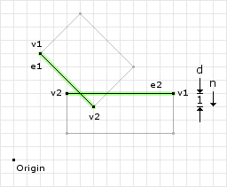
Figure 7 highlights the “best” edges on the shapes. Once we have found the edges we need to determine which edge is the reference edge and which is the incident edge:

e1 = (2, 8) to (6, 4)  = (6, 4) - (2, 8)  = (4, -4)
e2 = (12, 5) to (4, 5) = (4, 5) - (12, 5) = (-8, 0)
e1Dotn = (4, -4) · (0, -1) = 4
e2Dotn = (-8, 0) · (0, -1) = 0
// since the dot product is greater for e1 we will use
// e2 as the reference edge and set the flip variable
// to true
ref = e2;
inc = e1;
flip = true;

Now that we have identified the reference and incident edges we perform the first clipping operation:

ref.normalize() = (-1, 0)
o1 = (-1, 0) · (12, 5) = -12
// now we call clip with 
// v1 = inc.v1 = (2, 8)
// v2 = inc.v2 = (6, 4)
// n  = ref    = (-1, 0)
// o  = o1     = -12
d1 = (-1, 0) · (2, 8) - -12 = 10
d2 = (-1, 0) · (6, 4) - -12 = 6
// since both are greater than or equal
// to zero we add both to the clipped
// points object
cp.add(v1);
cp.add(v2);
// since both are positive then we skip
// the if block and return

Figure 8: The first clip of example 2

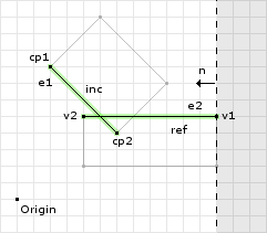
The first clipping operation did not remove any points. Figure 8 shows the clipping plane and the valid and invalid regions. Both points were found to be inside the valid region of the clipping plane. Now for the second clipping operation:

o1 = (-1, 0) · (4, 5) = -4
// now we call clip with 
// v1 = cp[0] = (2, 8)
// v2 = cp[1] = (6, 4)
// n  = ref   = (1, 0)
// o  = o1    = 4
d1 = (1, 0) · (2, 8) - 4 = -2
d2 = (1, 0) · (6, 4) - 4 = 2
// we only add v2 to the clipped points since
// its the only one that is greater than or
// equal to zero
cp.add(v2);
// since d1 * d2 = -4 we go into the if block
e = (6, 4) - (2, 8) = (4, -4)
u = -2 / (-2 - 2) = 1/2
e * u + v1 = (4 * 1/2, -4 * 1/2) + (2, 8) = (4, 6)
// then we add this point to the clipped points
cp.add(4, 6);

Figure 9: The second clip of example 2

The second clipping operation removed one point that was outside the clipping plane (i.e. past the offset). But since there was another point on the opposite side of the clipping plane, we compute a new point on the edge and use it as the second point of the result. See figure 9 for an illustration. Now we continue to the last clipping operation:

// compute the reference edge's normal
refNorm = (0, 1)
// since we flipped the reference and incident
// edges we need to negate refNorm
refNorm = (0, -1)
max = (0, -1) · (12, 5) = -5
// now we clip the points about this clipping plane, where:
// cp[0] = (6, 4)
// cp[1] = (4, 6)
(0, -1) · (6, 4) - -5 = 1
(0, -1) · (4, 6) - -5 = -1
// since the second point is negative we remove the point
// from the final list of contact points

Figure 10: The final clip of example 2

On the final clipping operation we remove one point. Figure 10 shows the final clipping operation and the valid region for the points. This ends the clipping operation returning a contact manifold of only one point.

// the collision manifold for example 2
cp[0] = (6, 4)
// removed because it was in the invalid region
cp[1] = null

Example 3
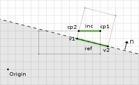
The last example will show the case where the contact point’s depth must be adjusted. In the previous two examples, the depth of the contact point has remained valid at 1 unit. For this example we will need to modify the psuedo code slightly. See figure 11.

Figure 11: A very common box-box collision

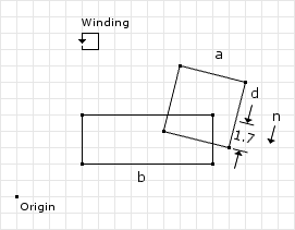
// from the collision detector
// separation normal and depth
normal = (-0.19, -0.98)
depth = 1.7

The first step is to get the “best” edges (the edges that are involved in the collision):

// the "best" edges    ( max ) | (  v1 ) | ( v2 )
//                    ---------+---------+-------
Edge e1 = A.best(n)  = ( 9, 4) | ( 9, 4) | (13, 3)
Edge e2 = B.best(-n) = (12, 5) | (12, 5) | (4, 5)

Figure 12: The “best” edges of figure 11

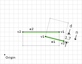
Figure 12 highlights the “best” edges on the shapes. Once we have found the edges we need to determine which edge is the reference edge and which is the incident edge:

e1 = (9, 4) to (13, 3)  = (13, 3) - (9, 4)  = (4, -1)
e2 = (12, 5) to (4, 5) = (4, 5) - (12, 5) = (-8, 0)
e1Dotn = (4, -1) · (-0.19, -0.98) = -0.22
e2Dotn = (-8, 0) · (-0.19, -0.98) =  1.52
// since the dot product is greater for e2 we will use
// e1 as the reference edge and set the flip variable
// to true
ref = e1;
inc = e2;

Now that we have identified the reference and incident edges we perform the first clipping operation:

ref.normalize() = (0.97, -0.24)
o1 = (0.97, -0.24) · (9, 4) = 7.77
// now we call clip with 
// v1 = inc.v1 = (12, 5)
// v2 = inc.v2 = (4, 5)
// n  = ref    = (0.97, -0.24)
// o  = o1     = 7.77
d1 = (0.97, -0.24) · (12, 5) - 7.77 = 2.67
d2 = (0.97, -0.24) · (4, 5)  - 7.77 = -5.09
// we only add v1 to the clipped points since
// its the only one that is greater than or
// equal to zero
cp.add(v1);
// since d1 * d2 = -13.5903 we go into the if block
e = (4, 5) - (12, 5) = (-8, 0)
u = 2.67 / (2.67 - -5.09) = 2.67/7.76
e * u + v1 = (-8 * 0.34, 0 * 0.34) + (12, 5) = (9.28, 5)
// then we add this point to the clipped points
cp.add(9.28, 5);

Figure 13: The first clip of example 3

The first clipping operation removed one point that was outside the clipping plane (i.e. past the offset). But since there was another point on the opposite side of the clipping plane, compute a new point on the edge and use it as the second point of the result. See figure 13 for an illustration.

Since we still have two points in the ClippedPoints object we can continue and perform the second clipping operation:

o2 = (0.97, -0.24) · (13, 3) = 11.89
// now we call clip with
// v1 = cp[0] = (12, 5)
// v2 = cp[1] = (9.28, 5)
// n  = -ref  = (-0.97, 0.24)
// o  = -o1   = -11.89
d1 = (-0.97, 0.24) · (12, 5)   - -11.89 = 1.45
d2 = (-0.97, 0.24) · (9.28, 5) - -11.89 = 4.09
// since both are greater than or equal
// to zero we add both to the clipped
// points object
cp.add(v1);
cp.add(v2);
// since both are positive then we skip
// the if block and return

Figure 14: The second clip of example 3

The second clipping operation did not remove any points. Figure 14 shows the clipping plane and the valid and invalid regions. Both points were found to be inside the valid region of the clipping plane. Now we continue to the last clipping operation:

// compute the reference edge's normal
refNorm = (0.24, 0.97)
// we didn't flip the reference and incident
// edges, so dont flip the reference edge normal
max = (0.24, 0.97) · (9, 4) = 6.04
// now we clip the points about this clipping plane, where:
// cp[0] = (12, 5)
// cp[1] = (9.28, 5)
(0.24, 0.97) · (12, 5)   - 6.04 = 1.69
(0.24, 0.97) · (9.28, 5) - 6.04 = 1.04
// both points are in the valid region so we keep them both

Figure 15: The final clip of example 3

On the final clipping operation we keep both of the points. Figure 15 shows the final clipping operation and the valid region for the points. This ends the clipping operation returning a contact manifold of two points.

// the collision manifold for example 3
cp[0] = (12, 5)
cp[1] = (9.28, 5)

The tricky bit here is the collision depth. The original depth of 1.7 that was computed by the collision detector is only valid for one of the points. If you were to use 1.7 for cp[1], you would over compensate the collision. So, because we may produce a new collision point, which is not a vertex on either shape, we must compute the depth of each of the points that we return. Thankfully, we have already done this when we test if the points are valid in the last clipping operation. The depth for the first point is 1.7, as originally found by the collision detector, and 1.04 for the second point.

// previous psuedo code
//if (refNorm.dot(cp[0]) - max < 0.0) {
//  cp[0].valid = false;
//}
//if (refNorm.dot(cp[1]) - max < 0.0) {
//  cp[1].valid = false;
//}
// new code, just save the depth
cp[0].depth = refNorm.dot(cp[0]) - max;
cp[1].depth = refNorm.dot(cp[1]) - max;
if (cp[0].depth < 0.0) {
  cp.remove(cp[0]);
}
if (cp[1].depth < 0.0) {
  cp.remove(cp[1]);
}

// the revised collision manifold for example 3
// point 1
cp[0].point = (12, 5)
cp[0].depth = 1.69
// point 2
cp[1].point = (9.28, 5)
cp[1].depth = 1.04

Curved Shapes
It’s apparent by now that this method relies heavily on edge features. This poses a problem for curved shapes like circles since their edge(s) aren’t represented by vertices. Handling circles can be achieved by simply get the farthest point in the circle, instead of the farthest edge, and using the single point returned as the contact manifold. Capsule shapes can do something similar when the farthest feature is inside the circular regions of the shape, and return an edge when its not.

Alternative Methods
An alternative method to clipping is to opt for the expanded shapes route that was discussed in the GJK/EPA posts. The original shapes are expaned/shrunk so that the GJK distance method can be used to detect collisions and obtain the MTV. Since GJK is being used, you can also get the closest points. The closest points can be used to obtain one collision point ().

Since GJK only gives one collision point per detection, and usually more than one is required (especially for physics), we need to do something else to obtain the other point(s). The following two methods are the most popular:

1. Cache the points from this iteration and subsequent ones until you have enough points to make a acceptable contact manifold.
2. Perturb the shapes slightly to obtain more points.

Caching is used by the popular physics engine and entails saving contact points over multiple iterations and then applying a reduction algorithm once a certain number of points has been reached. The reduction algorithm will typically keep the point of maximum depth and a fixed number of points. The points retained, other than the maximum depth point, will be the combination of points that maximize the contact area.

Perturbing the shapes slightly allows you to obtain all the contact points necessary on every iteration. This causes the shapes to be collision detected many times each iteration instead of once per iteration.

Skip to about 2 minutes in to skip the random motorcycle stuff at the beginning.

1. Problem Definition
2. Process Overview
3. The Jacobian
4. Compute The K Matrix

Problem Definition
It’s probably good to start with a good definition of what we are trying to accomplish.

We want to take two or more bodies and constrain their motion in some way. For instance, say we want two bodies to only be able to rotate about a common point (Revolute Joint). The most common application are constraints between pairs of bodies. Because we have constrained the motion of the bodies, we must find the correct velocities, so that constraints are satisfied otherwise the integrator would allow the bodies to move forward along their current paths. To do this we need to create equations that allow us to solve for the velocities.

What follows is the derivation of the equations needed to solve for a Prismatic constraint.

Process Overview
Let’s review the process:

1. Create a position constraint equation.
2. Perform the derivative with respect to time to obtain the velocity constraint.
3. Isolate the velocity.

Using these steps we can ensure that we get the correct velocity constraint. After isolating the velocity we inspect the equation to find J, the Jacobian.

Most constraint solvers today solve on the velocity level. Earlier work solved on the acceleration level.

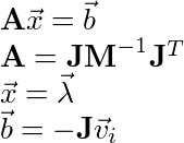
Once the Jacobian is found we use that to compute the K matrix. The K matrix is the A in the Ax = b general form equation.

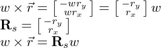
The Jacobian
As earlier stated, the Prismatic Joint is just like the Line Joint only it does not allow rotation about the anchor point. Because of this, we can formulate the Prismatic Joint by combining two joints: Line Joint and Angle Joint. This allows us to skip directly to the Jacobian:

See the “Line Constraint” and “Angle Constraint” posts for the derivation of their Jacobians.

Compute The K Matrix
Lastly, to solve the constraint we need to compute the values for A (I use the name K) and b:

See the “Equality Constraints” post for the derivation of the A matrix and b vector.

The b vector is fairly straight forward to compute. Therefore I’ll skip that and compute the K matrix symbolically:

Multiplying left to right the first two matrices we obtain:

Multiplying left to right again:

If we use the following just to clean things up:

We get:

And if t is normalized we get:

Plug the values of the K matrix and b vector into your linear equation solver and you will get the impulse required to satisfy the constraint.

Note here that if you are using an iterative solver that the K matrix does not change over iterations and as such can be computed once each time step.

Another interesting thing to note is that the K matrix will always be a square matrix with a size equal to the number of degrees of freedom (DOF) removed. This is a good way to check that the derivation was performed correctly.

There is a great open source project called that makes the OpenGL API available to Java.

You can test out the new TestBed .

In addition to the full OpenGL API, JOGL also offers OO approaches to common tasks like texturing, shaders, etc. The project owners, after reviving JOGL and JOAL (thank you!!!) have also been working on a binding to OpenCL called JOCL. This seems very promising and hopefully I’ll have some time to actually look into using this to help speed up some bottlenecks in dyn4j.

As a side note, I do have to say that the OpenGL API is really good and pretty well documented. I had a few “scratch my head” moments but for the most part I’m really liking it.

1. Problem Definition
2. Process Overview
3. Position Constraint
4. The Derivative
5. Isolate The Velocities
6. Compute The K Matrix

Problem Definition
It’s probably good to start with a good definition of what we are trying to accomplish.

We want to take two or more bodies and constrain their motion in some way. For instance, say we want two bodies to only be able to rotate about a common point (Revolute Joint). The most common application are constraints between pairs of bodies. Because we have constrained the motion of the bodies, we must find the correct velocities, so that constraints are satisfied otherwise the integrator would allow the bodies to move forward along their current paths. To do this we need to create equations that allow us to solve for the velocities.

What follows is the derivation of the equations needed to solve for a Line constraint.

Process Overview
Let’s review the process:

1. Create a position constraint equation.
2. Perform the derivative with respect to time to obtain the velocity constraint.
3. Isolate the velocity.

Using these steps we can ensure that we get the correct velocity constraint. After isolating the velocity we inspect the equation to find J, the Jacobian.

Most constraint solvers today solve on the velocity level. Earlier work solved on the acceleration level.

Once the Jacobian is found we use that to compute the K matrix. The K matrix is the A in the Ax = b general form equation.

Position Constraint
So the first step is to write out an equation that describes the constraint. A Line Joint should allow the two bodies to only translate along a given line, but should allow them to rotate about an anchor point. In other words:

where:

If we examine the equation we can see that this will allow us to constraint the linear motion. This equation states that any motion that is not along the vector u is invalid, because the tangent of that motion projected onto (via the dot product) the u vector will no longer yield 0.

The initial vector u will be supplied in the construction of the constraint. From u, we will obtain the tangent of u, the t vector. Each simulation step we will recompute u from the anchor points and use it along with the saved t vector to determine if the constraint has been violated.

Notice that this does not constrain the rotation of the bodies about the anchor point however. To also constrain the rotation about the anchor point use a prismatic joint.

The Derivative
The next step after defining the position constraint is to perform the derivative with respect to time. This will yield us the velocity constraint.

The velocity constraint can be found/identified directly, however its encouraged that a position constraint be created first and a derivative be performed to ensure that the velocity constraint is correct.

Another reason to write out the position constraint is because it can be useful during whats called the position correction step; the step to correct position errors (drift).

By the chain rule:

Where the derivative of u:

The derivative of a fixed length vector under a rotation frame is the cross product of the angular velocity with that fixed length vector.

And the derivative of t:

Here is one tricky part about this derivation. We know that t, like r in the u derivation, is a fixed length vector under a rotation frame. A vector can only be fixed in one coordinate frame, therefore you must choose one: a or b. I chose b, but either way, as long as the K matrix and b vector derivations are correct it will still solve the constraint.

Substituting these back into the equation creates:

Now we need to distribute, and on the last term I’m going to use the property that dot products are commutative:

Now we need to group like terms, but the terms are jumbled. We can use the identity:

and the property that dot products are commutative to obtain:

Now we can use the property that the cross product is anti-commutative on the last term to obtain the following. Then we group by like terms:

Isolate The Velocities
The next step involves isolating the velocities and identifying the Jacobian. This may be confusing at first because there are two velocity variables. In fact, there are actually four, the linear and angular velocities of both bodies. To isolate the velocities we will need to employ some identities and matrix math.

All the velocity terms are already ready to be isolated, by employing some matrix math we can obtain:

By inspection the Jacobian is:

Compute The K Matrix
Lastly, to solve the constraint we need to compute the values for A (I use the name K) and b:

See the “Equality Constraints” post for the derivation of the A matrix and b vector.

The b vector is fairly straight forward to compute. Therefore I’ll skip that and compute the K matrix symbolically:

Multiplying left to right the first two matrices we obtain:

Multiplying left to right again:

Plug the values of the K matrix and b vector into your linear equation solver and you will get the impulse required to satisfy the constraint.

Note here that if you are using an iterative solver that the K matrix does not change over iterations and as such can be computed once each time step.

Another interesting thing to note is that the K matrix will always be a square matrix with a size equal to the number of degrees of freedom (DOF) removed. This is a good way to check that the derivation was performed correctly.

This post will differ slightly from the previous posts. A weld joint is basically a revolute joint + an angle joint. In that case we can use the resulting Jacobians from those posts to skip a bit of the work.

1. Problem Definition
2. Process Overview
3. The Jacobian
4. Compute The K Matrix

Problem Definition
It’s probably good to start with a good definition of what we are trying to accomplish.

We want to take two or more bodies and constrain their motion in some way. For instance, say we want two bodies to only be able to rotate about a common point (Revolute Joint). The most common application are constraints between pairs of bodies. Because we have constrained the motion of the bodies, we must find the correct velocities, so that constraints are satisfied otherwise the integrator would allow the bodies to move forward along their current paths. To do this we need to create equations that allow us to solve for the velocities.

What follows is the derivation of the equations needed to solve for a Weld constraint.

Process Overview
Let’s review the process:

1. Create a position constraint equation.
2. Perform the derivative with respect to time to obtain the velocity constraint.
3. Isolate the velocity.

Using these steps we can ensure that we get the correct velocity constraint. After isolating the velocity we inspect the equation to find J, the Jacobian.

Most constraint solvers today solve on the velocity level. Earlier work solved on the acceleration level.

Once the Jacobian is found we use that to compute the K matrix. The K matrix is the A in the Ax = b general form equation.

The Jacobian
Like stated above, the weld constraint is just a combination of two other constraints: point-to-point and angle constraints. As such, we can simply combine the Jacobians we found for those constraints into one Jacobain:

See the “Point-to-Point Constraint” and “Angle Constraint” posts for the derivation of their Jacobians.

Compute The K Matrix
Lastly, to solve the constraint we need to compute the values for A (I use the name K) and b:

See the “Equality Constraints” post for the derivation of the A matrix and b vector.

For this constraint the b vector computation isn’t as simple as in past constraints. So I’ll work this out as well:

Notice here that the first element in the b vector is a vector also. This makes the b vector a 3×1 vector instead of the normal 2×1 that we have seen thus far.

Now on to computing the K matrix:

Multiplying left to right the first two matrices we obtain:

Multiplying left to right again:

Unlike previous posts, some of the elements in the above matrix are matrices themselves. When we multiply out the elements we’ll see that the resulting K matrix is actually a 3×3 matrix.

It makes sense that the K matrix is a 3×3 because the b vector was a 3×1, meaning we have 3 variables to solve for. The b vector and K matrix dimensions must match.

So lets take each element and work them out separately, starting with the first element. We can actually copy the result from the Point-to-Point constraint post since its exactly the same:

Now let move on to the second element. If we remember:

So multiplying and adding the vectors here yields the matrix:

Likewise, for the third element:

Lastly the last element can be left as is since its just a scalar.

Now adding all these elements back into one big matrix we obtain:

Plug the values of the K matrix and b vector into your linear equation solver and you will get the impulse required to satisfy the constraint.

Note here that if you are using an iterative solver that the K matrix does not change over iterations and as such can be computed once each time step.

Another interesting thing to note is that the K matrix will always be a square matrix with a size equal to the number of degrees of freedom (DOF) removed. This is a good way to check that the derivation was performed correctly.

1. Problem Definition
2. Process Overview
3. Position Constraint
4. The Derivative
5. Isolate The Velocities
6. Compute The K Matrix

Problem Definition
It’s probably good to start with a good definition of what we are trying to accomplish.

We want to take two or more bodies and constrain their motion in some way. For instance, say we want two bodies to only be able to rotate about a common point (Revolute Joint). The most common application are constraints between pairs of bodies. Because we have constrained the motion of the bodies, we must find the correct velocities, so that constraints are satisfied otherwise the integrator would allow the bodies to move forward along their current paths. To do this we need to create equations that allow us to solve for the velocities.

What follows is the derivation of the equations needed to solve for an Angle constraint.

Process Overview
Let’s review the process:

1. Create a position constraint equation.
2. Perform the derivative with respect to time to obtain the velocity constraint.
3. Isolate the velocity.

Using these steps we can ensure that we get the correct velocity constraint. After isolating the velocity we inspect the equation to find J, the Jacobian.

Most constraint solvers today solve on the velocity level. Earlier work solved on the acceleration level.

Once the Jacobian is found we use that to compute the K matrix. The K matrix is the A in the Ax = b general form equation.

Position Constraint
So the first step is to write out an equation that describes the constraint. An Angle Joint should allow the two bodies to move and freely, but should keep their rotations the same. In other words:

which says that the rotation about the center of body a minus the rotation about the center of body b should equal the initial reference angle calculated when the joint was created.

The Derivative
The next step after defining the position constraint is to perform the derivative with respect to time. This will yield us the velocity constraint.

The velocity constraint can be found/identified directly, however its encouraged that a position constraint be created first and a derivative be performed to ensure that the velocity constraint is correct.

Another reason to write out the position constraint is because it can be useful during whats called the position correction step; the step to correct position errors (drift).

As a side note, this is one of the easiest constraints to both derive and implement.

Start by taking the derivative of the position constraint:

Isolate The Velocities
The next step involves isolating the velocities and identifying the Jacobian. This may be confusing at first because there are two angular velocity variables. To isolate the velocities we will need to employ some matrix math.

Notice that I still included the linear velocities in the equation even though they are not present. This is necessary since the mass matrix is a 4×4 matrix so that we can multiply the matrices in the next step.

Now, by inspection, we obtain the Jacobian:

Compute The K Matrix
Lastly, to solve the constraint we need to compute the values for A (I use the name K) and b:

See the “Equality Constraints” post for the derivation of the A matrix and b vector.

The b vector is fairly straight forward to compute. Therefore I’ll skip that and compute the K matrix symbolically:

Multiplying left to right the first two matrices we obtain:

Multiplying left to right again:

Plug the values of the K matrix and b vector into your linear equation solver and you will get the impulse required to satisfy the constraint.

Note here that if you are using an iterative solver that the K matrix does not change over iterations and as such can be computed once each time step.

Another interesting thing to note is that the K matrix will always be a square matrix with a size equal to the number of degrees of freedom (DOF) removed. This is a good way to check that the derivation was performed correctly.

1. Problem Definition
2. Process Overview
3. Position Constraint
4. The Derivative
5. Isolate The Velocities
6. Compute The K Matrix

Problem Definition
It’s probably good to start with a good definition of what we are trying to accomplish.

We want to take two or more bodies and constrain their motion in some way. For instance, say we want two bodies to only be able to rotate about a common point (Revolute Joint). The most common application are constraints between pairs of bodies. Because we have constrained the motion of the bodies, we must find the correct velocities, so that constraints are satisfied otherwise the integrator would allow the bodies to move forward along their current paths. To do this we need to create equations that allow us to solve for the velocities.

What follows is the derivation of the equations needed to solve for a Pulleyconstraint.

Process Overview
Let’s review the process:

1. Create a position constraint equation.
2. Perform the derivative with respect to time to obtain the velocity constraint.
3. Isolate the velocity.

Using these steps we can ensure that we get the correct velocity constraint. After isolating the velocity we inspect the equation to find J, the Jacobian.

Most constraint solvers today solve on the velocity level. Earlier work solved on the acceleration level.

Once the Jacobian is found we use that to compute the K matrix. The K matrix is the A in the Ax = b general form equation.

Position Constraint
So the first step is to write out an equation that describes the constraint. A Distance Joint should allow the two bodies to move and rotate freely, but should keep them at a certain distance from one another. For a Pulley Joint its similar except that the bodes distance is constrained to two axes. In the middle we will allow the option of a block-and-tackle. Examining the image to the right, we see that there are two bodies: Ba, Bb who have distance constraints that are along axes: Ua, Ub which were formed from the Ground and Body anchor points: GAa, GAb, BAa, BAb.

Given this definition we can see that the direction of Ua and Ub can change if the bodies swing left or right for example.

Unlike the Distance Joint, a Pulley Joint allows the distances from the ground anchors to the body anchors to increase and decrease (the magnitude of Ua and Ub can also change). However, the total distance along the two axes must be equal to the initial distance when the joint was created (this is what we are trying to constrain). If we apply some scalar factor (or ratio) to the distances we can simulate a block-and-tackle.

We can represent this constraint by the following equation:

Where:

Where are the length of Ua, body a’s body anchor point, body a’s ground anchor point, and the vector Ua respectively.

Likewise are the length of Ub, body b’s body anchor point, body b’s ground anchor point, and the vector Ub respectively.

is computed once when the joint is created to obtain the target total length of the pulley.

Finally is a scalar ratio value that will allow us to simulate a block-and-tackle.

To review, our position constraint calculates the current lengths of the two axes (applying the ratio to one) and subtracts it from the initial to find how much the constraint is violated.

The Derivative
The next step after defining the position constraint is to perform the derivative with respect to time. This will yield us the velocity constraint.

The velocity constraint can be found/identified directly, however its encouraged that a position constraint be created first and a derivative be performed to ensure that the velocity constraint is correct.

Another reason to write out the position constraint is because it can be useful during whats called the position correction step; the step to correct position errors (drift).

Taking the derivative of our position constraint we get:

Then just to clean up a bit:

Now we need to perform the derivative on . If we remember was defined as:

So let’s side step for a minute and perform the derivative of :

We needed to use the chain rule in order to fully compute the derivative where the derivative of u:

The derivative of a fixed length vector under a rotation frame is the cross product of the angular velocity with that fixed length vector.

Note here that the g vector (ground anchor) is constant and therefore becomes the zero vector.

In the last few steps I replaced a portion of the equation with:

In addition, I replaced the dot product with a matrix multiplication by:

Now if we substitute back into the original equation we get:

Isolate The Velocities
The next step involves isolating the velocities and identifying the Jacobian. This may be confusing at first because there are two velocity variables. In fact, there are actually four, the linear and angular velocities of both bodies. To isolate the velocities we will need to employ some identities and matrix math.

The linear velocities are already isolated so we can ignore those for now. The angular velocities on the other hand have a pesky cross product. In 3D, we can use the identity that a cross product of two vectors is the same as the multiplication by a skew symmetric matrix and the other vector; see . For 2D, we can do something similar by examining the cross product itself:

Remember that the angular velocity in 2D is a scalar.

Removing the cross products using the process above yields:

Now, just to clean up some, if we inspect:

Now replacing what we found above into the original equation (and some clean up):

Now if we employ some matrix multiplication we can separate the velocities from the known coefficients:

Now, by inspection, we obtain the Jacobian:

Compute The K Matrix
Lastly, to solve the constraint we need to compute the values for A (I use the name K) and b:

See the “Equality Constraints” post for the derivation of the A matrix and b vector.

The b vector is fairly straight forward to compute. Therefore I’ll skip that and compute the K matrix symbolically:

Multiplying left to right the first two matrices we obtain:

Multiplying left to right again:

If we simplify using:

Remember the inertia tensor in 2D is a scalar, therefore we can pull it out to the front of the multiplications.

Plug the values of the K matrix and b vector into your linear equation solver and you will get the impulse required to satisfy the constraint.

Note here that if you are using an iterative solver that the K matrix does not change over iterations and as such can be computed once each time step.

Another interesting thing to note is that the K matrix will always be a square matrix with a size equal to the number of degrees of freedom (DOF) removed. This is a good way to check that the derivation was performed correctly.