After the first release of the project, I felt that it would be good to pass along what I learned about constrained dynamics.

This is not an easy subject and aside from purchasing books there’s not much information out there about it for those of us not accustomed to reading research papers or theses.

In this post I plan to solve a velocity constraint generally. Later posts will be for the individual types of constraints.

A phyiscial constraint is defined by some function:

Where x is the position of the body and R is the rotation of the body. Typically constraints are pairwise. You can formulate constraints using any number of bodies, however, pairwise formulations are simple. When this function is equal to zero the constraint is satisfied.

If we perform the derivative with respect to time we get the velocity constraint

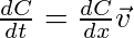
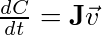
Since C is a function of positions and rotations who are themselves functions of time, we must perform the chain rule. The derivative of one vector function (C) by another vector function (x) yields a Jacobian matrix:

[1]

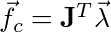
Where v is the vector of velocities from the bodies. The Jacobian rows contain the gradients of the scalar components of the constraint function C. We know that the gradient direction is the highest rate of increase of the scalar function C and unless the constraint is satisfied then it will be non-zero. Therefore the gradient is the direction of the illegal movement. We want the constraint force to act in this direction since we don’t want to constrain legal movement:

[2]

Where lambda a vector of the magnitudes of the constraint forces. The constraint force is the force that must be applied to counter act external forces so that the constraint is satisfied.

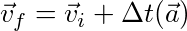
We know that the final velocity of a system is:

We also know that the sum of all the forces on a body is:

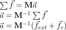
We can split the external forces and the constraint forces apart and then distribute:

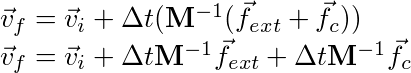
If we look closely we can perform the integration using the external forces separately therefore removing the external forces from the equation:

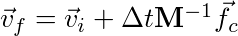[3]

Now if we substitute equation [2] into [3]:

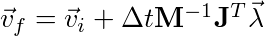[4]

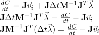
Now if we substitue equation [4] into equation [1]:

[5]

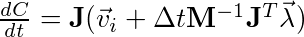
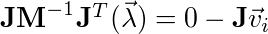
Now if we rearrange the terms to match the form Ax = b:

We also know that:

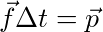
Where P is the impulse, therefore:

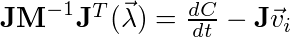[6]

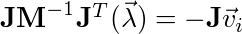
Where lambda is the constraint impulse. We stated at the beginning of the post that if the constraint is satisfied if the constraint equals zero. This is true for the velocity constraint as well:

This will solve the constraint exactly, however, given that the integrator is only an approximation of the ODE and the lack of infinite precision the constraint will “drift.” For example, a point-to-point constraint (simulates a revolute joint) will drift, where the local points of the world space anchor point slowly separate over time.

Drift can be solve using methods like Baumgarte stabilization, post/pre stabilizations methods, etc. That will be left for another post.

The equation is now in the form:

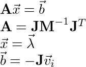
and can be solved using any linear equation solver desired. After solving for lamda, we can substitute it back into equation 4:

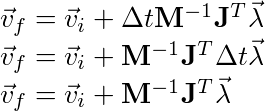
to find the final velocities.

Remember that the velocity vector is the velocity of the system and the mass matrix is the mass of the system. For example, a two body system would have the form:

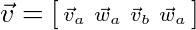
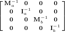
The Jacobian, as we will see in the next few posts, will be specific to the type of constraint being added and the number of bodies involved (as we see above).