Many have asked “How do I get the contact points from GJK?” or similar on the SAT, GJK, and EPA posts. I’ve finally got around to creating a post on this topic. Contact point generation is a vital piece of many applications and is usually the next step after collision detection. Generating good contact points is crucial to predictable and life-like iteractions between bodies. In this post I plan to cover a clipping method that is used in and . This is not the only method available and I plan to comment about the other methods near the end of the post.

1. Introduction
2. Finding the Features
3. Clipping
4. Example 1
5. Example 2
6. Example 3
7. Curved Shapes
8. Alternative Methods

Introduction
Most collision detection algorithms will return a separation normal and depth. Using this information we can translate the shapes directly to resolve the collision. Doing so does not exhibit real world physical behavior. As such, this isn’t sufficent for applications that want to model the physical world. To model real world iteractions effectively, we need to know where the collision occurred.

Contact points are usually world space points on the colliding shapes/bodies that represent where the collision is taking place. In the real world this would on the edge of two objects where they are touching. However, most simulations run collision detection routines on some interval allowing the objects overlap rather than touch. In this very common scenario, we must infer what the contact(s) should be.

More than one contact point is typically called a contact manifold or contact patch.

Finding the Features
The first step is to identify the features of the shapes that are involved in the collision. We can find the collision feature of a shape by finding the farthest vertex in the shape. Then, we look at the adjacent two vertices to determine which edge is the “closest.” We determine the closest as the edge who is most perpendicular to the separation normal.

// step 1
// find the farthest vertex in
// the polygon along the separation normal
int c = vertices.length;
for (int i = 0; i < c; i++) {
  double projection = n.dot(v);
  if (projection > max) {
    max = projection;
    index = i;
  }
}

// step 2
// now we need to use the edge that
// is most perpendicular, either the
// right or the left
Vector2 v = vertices[index];
Vector2 v1 = v.next;
Vector2 v0 = v.prev;
// v1 to v
Vector2 l = v - v1;
// v0 to v
Vector2 r = v - v0;
// the edge that is most perpendicular
// to n will have a dot product closer to zero
if (r.dot(n) <= l.dot(n)) {
  // the right edge is better
  // make sure to retain the winding direction
  return new Edge(v, v0, v);
} else {
  // the left edge is better
  // make sure to retain the winding direction
  return new Edge(v, v, v1);
}
// we return the maximum projection vertex (v)
// and the edge points making the best edge (v and either v0 or v1)

Be careful when computing the left and right (l and r in the code above) vectors as they both must point towards the maximum point. If one doesn’t that edge may always be used since its pointing in the negative direction and the other is pointing in the positive direction.

To obtain the correct feature we must know the direction of the separation normal ahead of time. Does it point from A to B or does it point from B to A? Its recommended that this is fixed, so for this post we will assume that the separation normal always points from A to B.

// find the "best" edge for shape A
Edge e1 = A.best(n);
// find the "best" edge for shape B
Edge e2 = B.best(-n);

Clipping
Now that we have the two edges involved in the collision, we can do a series of line/plane clips to get the contact manifold (all the contact points). To do so we need to identify the reference edge and incident edge. The reference edge is the edge most perpendicular to the separation normal. The reference edge will be used to clip the incident edge vertices to generate the contact manifold.

Edge ref, inc;
boolean flip = false;
if (e1.dot(n) <= e2.dot(n)) {
  ref = e1;
  inc = e2;
} else {
  ref = e2;
  inc = e1;
  // we need to set a flag indicating that the reference
  // and incident edge were flipped so that when we do the final
  // clip operation, we use the right edge normal
  flip = true;
}

Now that we have identified the reference and incident edges we can begin clipping points. First we need to clip the incident edge’s points by the first vertex in the reference edge. This is done by comparing the offset of the first vertex along the reference vector with the incident edge’s offsets. Afterwards, the result of the previous clipping operation on the incident edge is clipped again using the second vertex of the reference edge. Finally, we check if the remaining points are past the reference edge along the reference edge’s normal. In all, we perform three clipping operations.

ref.normalize();

double o1 = ref.dot(ref.v1);
// clip the incident edge by the first
// vertex of the reference edge
ClippedPoints cp = clip(inc.v1, inc.v2, ref, o1);
// if we dont have 2 points left then fail
if (cp.length < 2) return;

// clip whats left of the incident edge by the
// second vertex of the reference edge
// but we need to clip in the opposite direction
// so we flip the direction and offset
double o2 = ref.dot(ref.v2);
ClippedPoints cp = clip(cp[0], cp[1], -ref, -o2);
// if we dont have 2 points left then fail
if (cp.length < 2) return;

// get the reference edge normal
Vector2 refNorm = ref.cross(-1.0);
// if we had to flip the incident and reference edges
// then we need to flip the reference edge normal to
// clip properly
if (flip) refNorm.negate();
// get the largest depth
double max = refNorm.dot(ref.max);
// make sure the final points are not past this maximum
if (refNorm.dot(cp[0]) - max < 0.0) {
  cp.remove(cp[0]);
}
if (refNorm.dot(cp[1]) - max < 0.0) {
  cp.remove(cp[1]);
}
// return the valid points
return cp;

And the clip method:

// clips the line segment points v1, v2
// if they are past o along n
ClippedPoints clip(v1, v2, n, o) {
  ClippedPoints cp = new ClippedPoints();
  double d1 = n.dot(v1) - o;
  double d2 = n.dot(v2) - o;
  // if either point is past o along n
  // then we can keep the point
  if (d1 >= 0.0) cp.add(v1);
  if (d2 >= 0.0) cp.add(v2);
  // finally we need to check if they
  // are on opposing sides so that we can 
  // compute the correct point
  if (d1 * d2 < 0.0) {
    // if they are on different sides of the
    // offset, d1 and d2 will be a (+) * (-)
    // and will yield a (-) and therefore be
    // less than zero
    // get the vector for the edge we are clipping
    Vector2 e = v2 - v1;
    // compute the location along e
    double u = d1 / (d1 - d2);
    e.multiply(u);
    e.add(v1);
    // add the point
    cp.add(e); 
  }
}

Even though all the examples use box-box collisions, this method will work for any convex polytopes. See the end of the post for details on handling curved shapes.

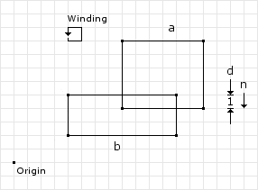
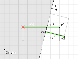
Example 1
Its best to start with a simple example explaining the process. Figure 1 shows a box vs. box collision with the collision information listed along with the winding direction of the vertices for both shapes. We have following data to begin with:

// from the collision detector
// separation normal and depth
normal = (0, -1)
depth = 1

The first step is to get the “best” edges, or the edges that are involved in the collision:

// the "best" edges    ( max ) | (  v1 ) | ( v2 )
//                    ---------+---------+-------
Edge e1 = A.best(n)  = ( 8, 4) | ( 8, 4) | (14, 4)
Edge e2 = B.best(-n) = (12, 5) | (12, 5) | ( 4, 5)

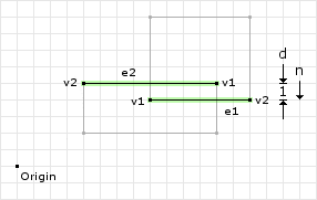
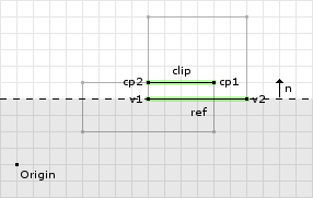
Figure 2 highlights the “best” edges on the shapes. Once we have found the edges, we need to determine which edge is the reference edge and which is the incident edge:

e1 = (8, 4) to (14, 4) = (14, 4) - (8, 4) = (6, 0)
e2 = (12, 5) to (4, 5) = (4, 5) - (12, 5) = (-8, 0)
e1Dotn = (6, 0) ·  (0, -1) = 0
e2Dotn = (-8, 0) · (0, -1) = 0
// since the dot product is the same we can choose either one
// using the first edge as the reference will let this example 
// be slightly simpler
ref = e1;
inc = e2;

Now that we have identified the reference and incident edges we perform the first clipping operation:

ref.normalize() = (1, 0)
o1 = (1, 0) · (8, 4) = 8
// now we call clip with 
// v1 = inc.v1 = (12, 5)
// v2 = inc.v2 = (4, 5)
// n  = ref    = (1, 0)
// o  = o1     = 8
d1 = (1, 0) · (12, 5) - 8 = 4
d2 = (1, 0) · (4, 5)  - 8 = -4
// we only add v1 to the clipped points since
// its the only one that is greater than or
// equal to zero
cp.add(v1);
// since d1 * d2 = -16 we go into the if block
e = (4, 5) - (12, 5) = (-8, 0)
u = 4 / (4 - -4) = 1/2
e * u + v1 = (-8 * 1/2, 0 * 1/2) + (12, 5) = (8, 5)
// then we add this point to the clipped points
cp.add(8, 5);

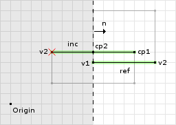
The first clipping operation removed one point that was outside the clipping plane (i.e. past the offset). But since there was another point on the opposite side of the clipping plane, we compute a new point on the edge and use it as the second point of the result. See figure 3 for an illustration.

Since we still have two points in the ClippedPoints object we can continue and perform the second clipping operation:

o2 = (1, 0) · (14, 4) = 14
// now we call clip with
// v1 = cp[0] = (12, 5)
// v2 = cp[1] = (8, 5)
// n  = -ref  = (-1, 0)
// o  = -o1   = -14
d1 = (-1, 0) · (12, 5) - -14 = 2
d2 = (-1, 0) · (8, 5)  - -14 = 6
// since both are greater than or equal
// to zero we add both to the clipped
// points object
cp.add(v1);
cp.add(v2);
// since both are positive then we skip
// the if block and return

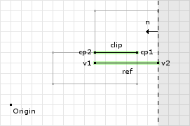
The second clipping operation did not remove any points. Figure 4 shows the clipping plane and the valid and invalid regions. Both points were found to be inside the valid region of the clipping plane. Now we continue to the last clipping operation:

// compute the reference edge's normal
refNorm = (0, 1)
// we didnt have to flip the reference and incident
// edges so refNorm stays the same
// compute the offset for this clipping operation
max = (0, 1) · (8, 4) = 4
// now we clip the points about this clipping plane, where:
// cp[0] = (12, 5)
// cp[1] = (8, 5)
(0, 1) · (12, 5) - 4 = 1
(0, 1) · (8, 5)  - 4 = 1
// since both points are greater than
// or equal to zero we keep them both

On the final clipping operation we keep both of the points. Figure 5 shows the final clipping operation and the valid region for the points. This ends the clipping operation returning a contact manifold of two points.

// the collision manifold for example 1
cp[0] = (12, 5)
cp[1] = (8, 5)

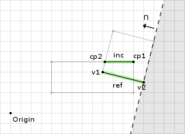
Example 2
The first example was, by far, the simplest. In this example we will see how the last clipping operation is used. Figure 6 shows two boxes in collision, but in a slightly different configuration. We have following data to begin with:

// from the collision detector
// separation normal and depth
normal = (0, -1)
depth = 1

The first step is to get the “best” edges (the edges that are involved in the collision):

// the "best" edges    ( max ) | (  v1 ) | ( v2 )
//                    ---------+---------+-------
Edge e1 = A.best(n)  = ( 7, 4) | ( 2, 8) | (6, 4)
Edge e2 = B.best(-n) = (12, 5) | (12, 5) | (4, 5)

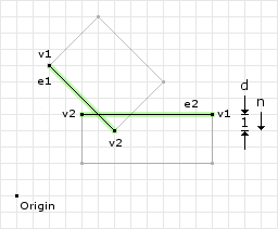
Figure 7 highlights the “best” edges on the shapes. Once we have found the edges we need to determine which edge is the reference edge and which is the incident edge:

e1 = (2, 8) to (6, 4)  = (6, 4) - (2, 8)  = (4, -4)
e2 = (12, 5) to (4, 5) = (4, 5) - (12, 5) = (-8, 0)
e1Dotn = (4, -4) · (0, -1) = 4
e2Dotn = (-8, 0) · (0, -1) = 0
// since the dot product is greater for e1 we will use
// e2 as the reference edge and set the flip variable
// to true
ref = e2;
inc = e1;
flip = true;

Now that we have identified the reference and incident edges we perform the first clipping operation:

ref.normalize() = (-1, 0)
o1 = (-1, 0) · (12, 5) = -12
// now we call clip with 
// v1 = inc.v1 = (2, 8)
// v2 = inc.v2 = (6, 4)
// n  = ref    = (-1, 0)
// o  = o1     = -12
d1 = (-1, 0) · (2, 8) - -12 = 10
d2 = (-1, 0) · (6, 4) - -12 = 6
// since both are greater than or equal
// to zero we add both to the clipped
// points object
cp.add(v1);
cp.add(v2);
// since both are positive then we skip
// the if block and return

The first clipping operation did not remove any points. Figure 8 shows the clipping plane and the valid and invalid regions. Both points were found to be inside the valid region of the clipping plane. Now for the second clipping operation:

o1 = (-1, 0) · (4, 5) = -4
// now we call clip with 
// v1 = cp[0] = (2, 8)
// v2 = cp[1] = (6, 4)
// n  = ref   = (1, 0)
// o  = o1    = 4
d1 = (1, 0) · (2, 8) - 4 = -2
d2 = (1, 0) · (6, 4) - 4 = 2
// we only add v2 to the clipped points since
// its the only one that is greater than or
// equal to zero
cp.add(v2);
// since d1 * d2 = -4 we go into the if block
e = (6, 4) - (2, 8) = (4, -4)
u = -2 / (-2 - 2) = 1/2
e * u + v1 = (4 * 1/2, -4 * 1/2) + (2, 8) = (4, 6)
// then we add this point to the clipped points
cp.add(4, 6);

The second clipping operation removed one point that was outside the clipping plane (i.e. past the offset). But since there was another point on the opposite side of the clipping plane, we compute a new point on the edge and use it as the second point of the result. See figure 9 for an illustration. Now we continue to the last clipping operation:

// compute the reference edge's normal
refNorm = (0, 1)
// since we flipped the reference and incident
// edges we need to negate refNorm
refNorm = (0, -1)
max = (0, -1) · (12, 5) = -5
// now we clip the points about this clipping plane, where:
// cp[0] = (6, 4)
// cp[1] = (4, 6)
(0, -1) · (6, 4) - -5 = 1
(0, -1) · (4, 6) - -5 = -1
// since the second point is negative we remove the point
// from the final list of contact points

On the final clipping operation we remove one point. Figure 10 shows the final clipping operation and the valid region for the points. This ends the clipping operation returning a contact manifold of only one point.

// the collision manifold for example 2
cp[0] = (6, 4)
// removed because it was in the invalid region
cp[1] = null

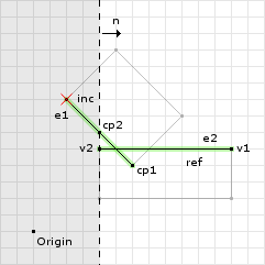
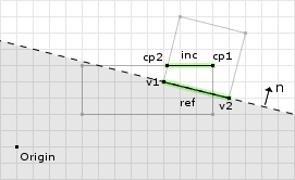
Example 3
The last example will show the case where the contact point’s depth must be adjusted. In the previous two examples, the depth of the contact point has remained valid at 1 unit. For this example we will need to modify the psuedo code slightly. See figure 11.

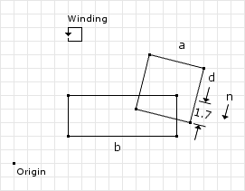
// from the collision detector
// separation normal and depth
normal = (-0.19, -0.98)
depth = 1.7

The first step is to get the “best” edges (the edges that are involved in the collision):

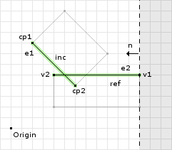
// the "best" edges    ( max ) | (  v1 ) | ( v2 )
//                    ---------+---------+-------
Edge e1 = A.best(n)  = ( 9, 4) | ( 9, 4) | (13, 3)
Edge e2 = B.best(-n) = (12, 5) | (12, 5) | (4, 5)

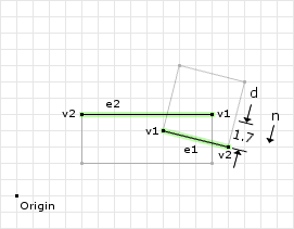
Figure 12 highlights the “best” edges on the shapes. Once we have found the edges we need to determine which edge is the reference edge and which is the incident edge:

e1 = (9, 4) to (13, 3)  = (13, 3) - (9, 4)  = (4, -1)
e2 = (12, 5) to (4, 5) = (4, 5) - (12, 5) = (-8, 0)
e1Dotn = (4, -1) · (-0.19, -0.98) = -0.22
e2Dotn = (-8, 0) · (-0.19, -0.98) =  1.52
// since the dot product is greater for e2 we will use
// e1 as the reference edge and set the flip variable
// to true
ref = e1;
inc = e2;

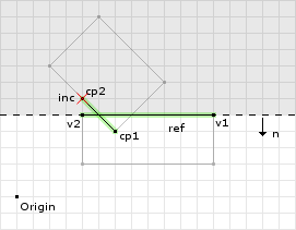
Now that we have identified the reference and incident edges we perform the first clipping operation:

ref.normalize() = (0.97, -0.24)
o1 = (0.97, -0.24) · (9, 4) = 7.77
// now we call clip with 
// v1 = inc.v1 = (12, 5)
// v2 = inc.v2 = (4, 5)
// n  = ref    = (0.97, -0.24)
// o  = o1     = 7.77
d1 = (0.97, -0.24) · (12, 5) - 7.77 = 2.67
d2 = (0.97, -0.24) · (4, 5)  - 7.77 = -5.09
// we only add v1 to the clipped points since
// its the only one that is greater than or
// equal to zero
cp.add(v1);
// since d1 * d2 = -13.5903 we go into the if block
e = (4, 5) - (12, 5) = (-8, 0)
u = 2.67 / (2.67 - -5.09) = 2.67/7.76
e * u + v1 = (-8 * 0.34, 0 * 0.34) + (12, 5) = (9.28, 5)
// then we add this point to the clipped points
cp.add(9.28, 5);

The first clipping operation removed one point that was outside the clipping plane (i.e. past the offset). But since there was another point on the opposite side of the clipping plane, compute a new point on the edge and use it as the second point of the result. See figure 13 for an illustration.

Since we still have two points in the ClippedPoints object we can continue and perform the second clipping operation:

o2 = (0.97, -0.24) · (13, 3) = 11.89
// now we call clip with
// v1 = cp[0] = (12, 5)
// v2 = cp[1] = (9.28, 5)
// n  = -ref  = (-0.97, 0.24)
// o  = -o1   = -11.89
d1 = (-0.97, 0.24) · (12, 5)   - -11.89 = 1.45
d2 = (-0.97, 0.24) · (9.28, 5) - -11.89 = 4.09
// since both are greater than or equal
// to zero we add both to the clipped
// points object
cp.add(v1);
cp.add(v2);
// since both are positive then we skip
// the if block and return

The second clipping operation did not remove any points. Figure 14 shows the clipping plane and the valid and invalid regions. Both points were found to be inside the valid region of the clipping plane. Now we continue to the last clipping operation:

// compute the reference edge's normal
refNorm = (0.24, 0.97)
// we didn't flip the reference and incident
// edges, so dont flip the reference edge normal
max = (0.24, 0.97) · (9, 4) = 6.04
// now we clip the points about this clipping plane, where:
// cp[0] = (12, 5)
// cp[1] = (9.28, 5)
(0.24, 0.97) · (12, 5)   - 6.04 = 1.69
(0.24, 0.97) · (9.28, 5) - 6.04 = 1.04
// both points are in the valid region so we keep them both

On the final clipping operation we keep both of the points. Figure 15 shows the final clipping operation and the valid region for the points. This ends the clipping operation returning a contact manifold of two points.

// the collision manifold for example 3
cp[0] = (12, 5)
cp[1] = (9.28, 5)

The tricky bit here is the collision depth. The original depth of 1.7 that was computed by the collision detector is only valid for one of the points. If you were to use 1.7 for cp[1], you would over compensate the collision. So, because we may produce a new collision point, which is not a vertex on either shape, we must compute the depth of each of the points that we return. Thankfully, we have already done this when we test if the points are valid in the last clipping operation. The depth for the first point is 1.7, as originally found by the collision detector, and 1.04 for the second point.

// previous psuedo code
//if (refNorm.dot(cp[0]) - max < 0.0) {
//  cp[0].valid = false;
//}
//if (refNorm.dot(cp[1]) - max < 0.0) {
//  cp[1].valid = false;
//}
// new code, just save the depth
cp[0].depth = refNorm.dot(cp[0]) - max;
cp[1].depth = refNorm.dot(cp[1]) - max;
if (cp[0].depth < 0.0) {
  cp.remove(cp[0]);
}
if (cp[1].depth < 0.0) {
  cp.remove(cp[1]);
}

// the revised collision manifold for example 3
// point 1
cp[0].point = (12, 5)
cp[0].depth = 1.69
// point 2
cp[1].point = (9.28, 5)
cp[1].depth = 1.04

Curved Shapes
It’s apparent by now that this method relies heavily on edge features. This poses a problem for curved shapes like circles since their edge(s) aren’t represented by vertices. Handling circles can be achieved by simply get the farthest point in the circle, instead of the farthest edge, and using the single point returned as the contact manifold. Capsule shapes can do something similar when the farthest feature is inside the circular regions of the shape, and return an edge when its not.

Alternative Methods
An alternative method to clipping is to opt for the expanded shapes route that was discussed in the GJK/EPA posts. The original shapes are expaned/shrunk so that the GJK distance method can be used to detect collisions and obtain the MTV. Since GJK is being used, you can also get the closest points. The closest points can be used to obtain one collision point ().

Since GJK only gives one collision point per detection, and usually more than one is required (especially for physics), we need to do something else to obtain the other point(s). The following two methods are the most popular:

1. Cache the points from this iteration and subsequent ones until you have enough points to make a acceptable contact manifold.
2. Perturb the shapes slightly to obtain more points.

Caching is used by the popular physics engine and entails saving contact points over multiple iterations and then applying a reduction algorithm once a certain number of points has been reached. The reduction algorithm will typically keep the point of maximum depth and a fixed number of points. The points retained, other than the maximum depth point, will be the combination of points that maximize the contact area.

Perturbing the shapes slightly allows you to obtain all the contact points necessary on every iteration. This causes the shapes to be collision detected many times each iteration instead of once per iteration.