In the last few posts we learned about using GJK for collision detection, distance between shapes, and finding the closest points. It was stated that GJK must be augmented, to find collision information like the penetration depth and vector, with another algorithm. One such algorithm is EPA.

I plan to cover the EPA algorithm and mention an alternative.

1. Introduction
2. Overview
3. Starting Point
4. Expansion
5. Example
6. Winding and Triple Product
7. Augmenting
8. Alternatives

Introduction
Like GJK, EPA uses the same concept of a Minkowski Sum, performing the difference operation instead of addition. Like the previous posts I will refer to this as the Minkowski Difference.

In the first GJK post we talked about how to determine if two convex shapes were intersecting; true or false. What we want to do now is after we determine that there is a collision, find the collision information: depth and vector.

Overview
In the GJK post we stated that we know the convex shapes are intersecting if the Minkowski Difference contains the origin. In addition to this, the distance from closest point on the Minkowski Difference to the origin is the penetration depth. Likewise, the vector from the closest point to the origin is the penetration vector.

Like GJK, EPA is an iterative algorithm. EPA stands for Expanding Polytope Algorithm and means just that. We want to create a polytope (or polygon) inside of the Minkowski Difference and iteratively expand it until we hit the edge of the Minkowski Difference. The key is to expand the closest feature to the origin of the polytope. If we perform this iteratively we will generate a polytope where the closest feature lies on the Minkowski Difference, thereby yeilding the penetration depth and vector.

EPA performs this task by using the same support function used in the other algorithms and the same notion of a simplex. One difference from GJK is that EPA’s simplex can have any number of points.

Starting Point
EPA needs an initial simplex to expand. The terminiation simplex from the GJK collision detection routine is a great start.

EPA needs a full simplex: Triangle for 2D and Tetrahedron for 3D. The GJK collision detection routine can be modified such that it always terminiates with the above cases. The GJK post will never terminiate, returning that the shapes are intersecting, until a triangle has been created.

Expansion
If we pass the termination simplex to EPA we can immediately start the expansion process:

Simplex s = // termination simplex from GJK
// loop to find the collision information
while (true) {
  // obtain the feature (edge for 2D) closest to the origin on the Minkowski Difference
  Edge e = findClosestEdge(s);
  // obtain a new support point in the direction of the edge normal
  Vector p = support(A, B, e.normal);
  // check the distance from the origin to the edge against the
  // distance p is along e.normal
  double d = p.dot(e.normal);
  if (d - e.distance < TOLERANCE) {
    // the tolerance should be something positive close to zero (ex. 0.00001)
  
    // if the difference is less than the tolerance then we can
    // assume that we cannot expand the simplex any further and
    // we have our solution
    normal = e.normal;
    depth = d;
  } else {
    // we haven't reached the edge of the Minkowski Difference
    // so continue expanding by adding the new point to the simplex
    // in between the points that made the closest edge
    simplex.insert(p, e.index);
  }
}

Where the findClosestEdge looks something like:

Edge closest = new Edge();
// prime the distance of the edge to the max
closest.distance = Double.MAX_VALUE;
// s is the passed in simplex
for (int i = 0; i < s.length; i++) {
  // compute the next points index
  int j = i + 1 == s.length ? 0 : i + 1;
  // get the current point and the next one
  Vector a = s.get(i);
  Vector b = s.get(j);
  // create the edge vector
  Vector e = b.subtract(a); // or a.to(b);
  // get the vector from the origin to a
  Vector oa = a; // or a - ORIGIN
  // get the vector from the edge towards the origin
  Vector n = Vector.tripleProduct(e, oa, e);
  // normalize the vector
  n.normalize();
  // calculate the distance from the origin to the edge
  double d = n.dot(a); // could use b or a here
  // check the distance against the other distances
  if (d < closest.distance) {
    // if this edge is closer then use it
    closest.distance = d;
    closest.normal = n;
    closest.index = j;
  }
}
// return the closest edge we found
return closest;

Example
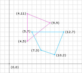
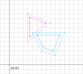
As always, I think its much easier to understand once you go through an example. We will use the example from the GJK post and determine the collision information using EPA.

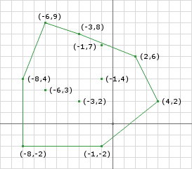
We start by supplying the GJK termination simplex to EPA:

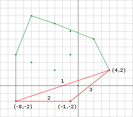
Iteration 1

Simplex s = {(4, 2), (-8, -2), (-1, -2)};
Edge closest = null;
{ // compute the closest edge
  // Edge 1
  a = (4, 2), b = (-8, -2)
  e = b - a = (-12, -4)
  oa = a = (4, 2)
  // triple product (A x B) x C = B(A.dot(C)) - A(B.dot(C))
  // oa(e.dot(e)) - e(oa.dot(e))
  n = (4, 2) * 160 - (-12, -4) * -56 = (640, 320) + (-672, -224) = (-32, 96)
  // normalize
  n ≈ (-32 / 101.19, 96 / 101.19) ≈ (-0.32, 0.95)
  d = a.dot(n) = 4 * -0.32 + 2 * 0.95 ≈ 0.62;
  
  // Edge 2
  a = (-8, -2), b = (-1, -2)
  e = b - a = (7, 0)
  oa = a = (-8, -2)
  // triple product (A x B) x C = B(A.dot(C)) - A(B.dot(C))
  // oa(e.dot(e)) - e(oa.dot(e))
  n = (-8, -2) * 49 - (7, 0) * -56 = (-392, -98) + (392, 0) = (0, -98)
  // normalize
  n = (0 / 98, -98 / 98) = (0, -1)
  d = a.dot(n) = -8 * 0 + -2 * -1 = 2;
  
  // Edge 3
  a = (-1, -2), b = (4, 2)
  e = b - a = (5, 4)
  oa = a = (-1, -2)
  // triple product (A x B) x C = B(A.dot(C)) - A(B.dot(C))
  // oa(e.dot(e)) - e(oa.dot(e))
  n = (-1, -2) * 41 - (5, 4) * -13 = (-41, -82) - (-65, -52) = (24, -30)
  // normalize
  n ≈ (24 / 38.42, -30 / 38.42) ≈ (0.62, -0.78)
  d = a.dot(n) = -1 * 0.62 + -2 * -0.78 ≈ 0.94;
  
  // we can see that Edge 1 is the closest, so...
  closest.normal = (-0.32, 0.95)
  closest.distance ≈ 0.62
  closest.index = 1;
}

// get a new support point in the direction of closest.normal
p = support(A, B, closest.normal) = (4, 11) - (10, 2) = (-6, 9)

// are we close enough?
dist = p.dot(closest.normal) = -6 * -0.32 + 9 * 0.95 = 1.92 + 8.55 = 10.47
// 10.47 - 0.62 = 9.85 obviously too big

// add it to the simplex at the index
s.add(p, closest.index)
// which makes s = {(4, 2), (-6, 9), (-8, -2), (-1, -2)};

Notice that we have expanded the simplex by adding another point. Its important to point out that the point we added is on the edge of the Minkowski Difference. Because all points that make up the simplex lie on the edge Minkowski Difference we can guarentee that the simplex is convex since the Minkowski Difference is convex. If the simplex was not convex then we wouldn’t be able to skip so many computations.

Another key that should be pointed out is how we add the new point to the simplex. We must add the new point in between the two points that create the closest edge. This way the shape stays convex. In this example the winding of the points doesn’t matter, however it is important to notice that insert the new point as we have done preserves the current winding direction. More on the simplex’s winding direction later…

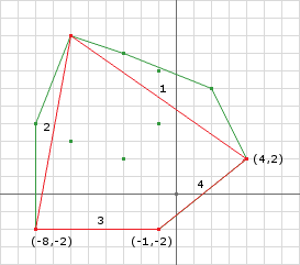
Iteration 2

Simplex s = {(4, 2), (-6, 9), (-8, -2), (-1, -2)};
Edge closest = null;
{ // compute the closest edge
  // Edge 1
  a = (4, 2), b = (-6, 9)
  e = b - a = (-10, 7)
  oa = a = (4, 2)
  // triple product (A x B) x C = B(A.dot(C)) - A(B.dot(C))
  // oa(e.dot(e)) - e(oa.dot(e))
  n = (4, 2) * 149 - (-10, 7) * -26 = (596, 298) + (-260, 182) = (336, 480)
  // normalize
  n ≈ (336 / 585.91, 480 / 585.91) ≈ (0.57, 0.82)
  d = a.dot(n) = 4 * 0.57 + 2 * 0.82 ≈ 3.92;
  
  // Edge 2
  a = (-6, 9), b = (-8, -2)
  e = b - a = (-2, -11)
  oa = a = (-6, 9)
  // triple product (A x B) x C = B(A.dot(C)) - A(B.dot(C))
  // oa(e.dot(e)) - e(oa.dot(e))
  n = (-6, 9) * 125 - (-2, -11) * -87 = (-750, 1125) + (-174, -957) = (-924, 168)
  // normalize
  n ≈ (-924 / 939.15, 168 / 939.15) ≈ (-0.98, 0.18)
  d = a.dot(n) = -6 * -0.98 + 9 * 0.18 ≈ 7.5;
  
  // Edge 3
  a = (-8, -2), b = (-1, -2)
  e = b - a = (7, 0)
  oa = a = (-8, -2)
  // triple product (A x B) x C = B(A.dot(C)) - A(B.dot(C))
  // oa(e.dot(e)) - e(oa.dot(e))
  n = (-8, -2) * 49 - (7, 0) * -56 = (-392, -98) + (392, 0) = (0, -98)
  // normalize
  n = (0 / 98, -98 / 98) = (0, -1)
  d = a.dot(n) = -8 * 0 + -2 * -1 = 2;
  
  // Edge 4
  a = (-1, -2), b = (4, 2)
  e = b - a = (5, 4)
  oa = a = (-1, -2)
  // triple product (A x B) x C = B(A.dot(C)) - A(B.dot(C))
  // oa(e.dot(e)) - e(oa.dot(e))
  n = (-1, -2) * 41 - (5, 4) * -13 = (-41, -82) - (-65, -52) = (24, -30)
  // normalize
  n ≈ (24 / 38.42, -30 / 38.42) ≈ (0.62, -0.78)
  d = a.dot(n) = -1 * 0.62 + -2 * -0.78 ≈ 0.94;
  
  // we can see that Edge 4 is the closest, so...
  closest.normal = (0.62, -0.78)
  closest.distance ≈ 0.94
  closest.index = 0;
}

// get a new support point in the direction of closest.normal
p = support(A, B, closest.normal) = (9, 9) - (5, 7) = (4, 2)

// are we close enough?
dist = p.dot(closest.normal) = 4 * 0.62 + 2 * -0.78 = 0.92
// 0.92 - 0.94 = 0.02 small enough!
// we exit the loop returning (0.62, -0.78) as the collision normal
// and 0.92 as the depth

In the second iteration we see that the closest edge of the simplex actually lies on the Minkowski Difference. We can see by inspection that Edge 4′s normal is the collision normal and that the perpendicular distance from the edge to the origin is the penetration depth. This is confirmed in the last iteration.

We terminated on the second iteration because the distance to the new simplex point was not more than the distance to the closest edge indicating that we cannot expand our simplex any futher. If higher precision numbers were used we would see that the value of the dist variable would be much closer to zero which makes sense since the new support point lies on the closest edge.

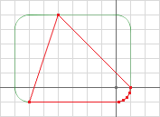
We still need to have a tolerance because of curved shapes and finite precision math. For a curved Minkowski Difference, the simplex will build smaller and smaller edges to conform to the curvature. You can see this in figure 5, however it may be many more edges because of the increase precision.

Winding and Triple Product
Earlier I mentioned something about the winding of the simplex being preserved. This is important to handle a special case of collisions.

Small or touching collisions can cause EPA problems which stem from the use of the triple product. If the origin lies really close to the closest edge the triple product may return a zero vector (because of finite precision). When we go to normalize the vector we will divide by zero: not good.

If we look at the reason we are using the triple product we come up with another method to fix this problem. The triple product is used to get the normal vector of an edge in the opposite direction of the origin. We can do the same thing by using the per-product of the edge.

The per-product is defined as:

if A = (x, y)
A.perproduct() = (-y, x) or (y, -x) depending on the
handedness of the coordinate system (right or left respectively)

In this instance the left or right handedness actually is determined by the winding of the simplex. If the winding of the simplex is counter-clockwise then we want to use the right per-product. Likewise if the simplex winding is clockwise then we want to use the left per-product. We can assume this because we have already guarenteed that the origin is contained in the simplex.

So instead of using the triple product we can use the per-product to get the normal of the edge no matter how close the origin is to the closest edge. The new code looks something like this:

// we change this
// Vector n = Vector.tripleProduct(e, oa, e);
// to this
if (winding == CLOCKWISE) {
  n = e.left(); // (y, -x)
} else {
  n = e.right(); // (-y, x)
}

It was important to note that the winding of the simplex is preserved because this means we can determine the winding of the simplex once making the new code more efficient and robust.

Augmenting
EPA is often not used for small penetrations because of the computational cost. Therefore you may see EPA supplemented with GJK penetration detection algorithm. To use GJK for collision information involves using smaller versions of the colliding shapes (called core shapes) and performing a GJK distance check. Once the distance between the core shapes is found, subtract it from the sum of the radial shinkage applied to the shapes.

Alternatives
There are alternatives to using EPA to determine collision information after GJK has detected a collision. I’m only going to mention one here: sampling for the smallest penetration.

Generate a sample of directions. Find the distance from the origin to the surface of the Minkowski Difference (like we do in EPA) along each direction. Use the one with the smallest distance.

This is obviously an estimation instead of an exact answer, however it can be improved by intelligent selection of the directions.

• Evenly distribute the directions along the unit circle/sphere
• Use more directions
• Use the edge normals of each shape
• Use the vector from center to center of the shapes
• etc.

For low vertex count polygons this may seem like more work, but for high vertex count polyhedrons it can be faster than EPA and still yield an acceptable result.

The above EPA implementation adds 22+ operations every time a new simplex point is added. This is significant when the Minkowski Difference has many vertices or has curved edges.